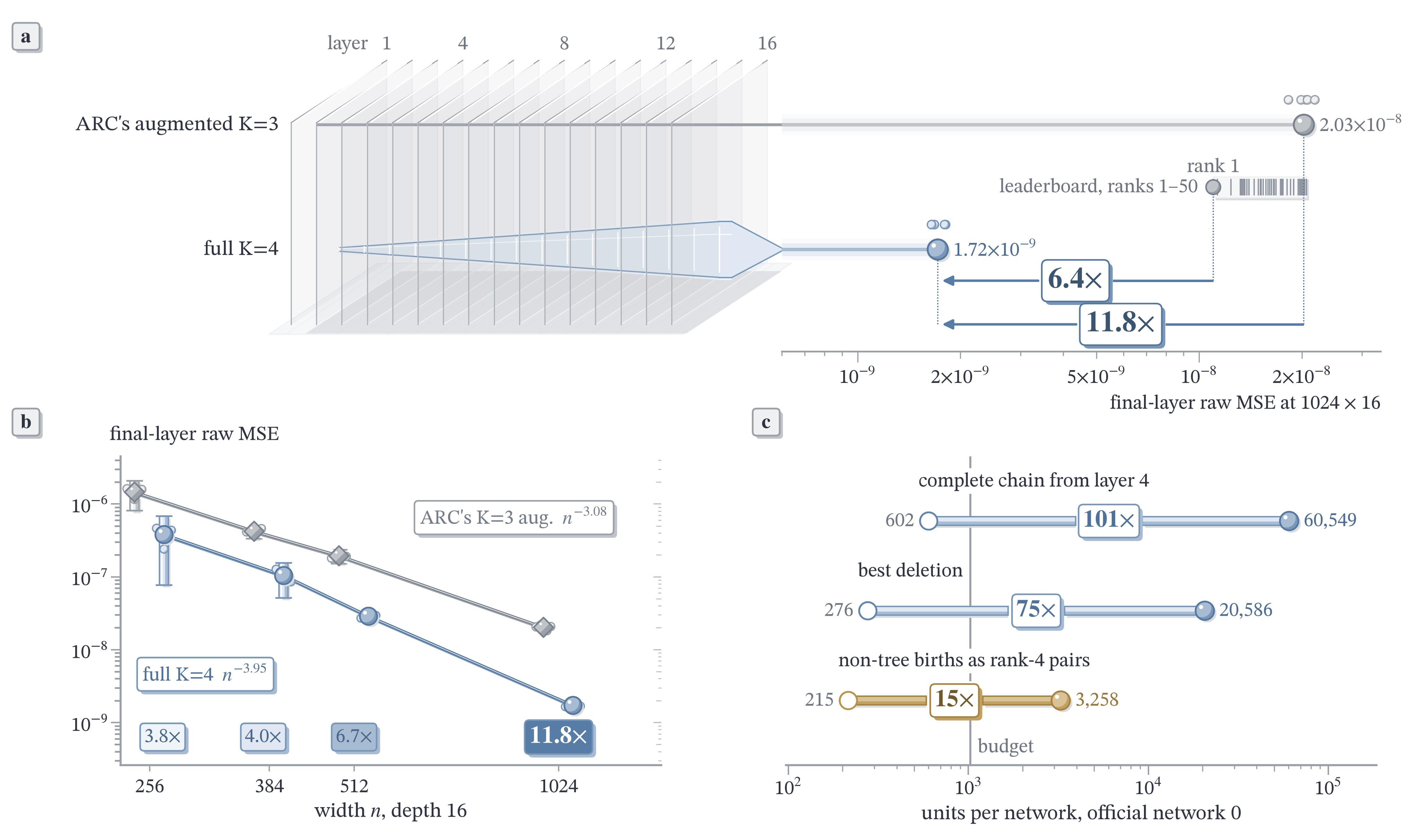
Figure 0. Exact unaugmented K=4 at 1024 × 16 ends 11.8× below augmented K=3 on all five official networks and 6.4× below the lowest raw error on the leaderboard, its error falling as n^−3.95.
Top: the 16 layers of the five official networks as glass plates; each beam ends at its final-layer MSE on one log ruler, ticked with every entry ranked 1–50 on the 18 October leaderboard, on its 50 networks. Bottom left: raw final MSE against width at depth 16, chips K=3 aug ÷ K=4 at each width. Bottom right: from layer 4 on official network 0, counted units (disc) against the units at which each configuration ties our scored chain (ring).
Full report (PDF, 28 pages) (1.3 MB) · code (MIT), every saved prediction and a script behind every number: GitHub - logxio/fourth-cumulant · GitHub
Submission ID: #336537. Graded 3.145e-9 adjusted (final-layer MSE 1.853e-8 at C/B 0.169), no failed networks. This write-up corresponds to that one submission; the other receipts below are its predecessors and its graded control, cited as evidence.
TL;DR. We ran ARC’s complete K=4 cumulant recursion at the challenge shape, 1024 × 16, the first public run at that size, with zero samples, zero fitted constants and no tuning. Phase 1 had found K=4 at a 61.5 GB memory wall already at 256 × 16 (18154), and 504aldo’s findings log advised stopping at K=3 for small n/L; the wall was storage, and the small-n/L loss was augmentation. Storing each source as its birth legs, its birth kernel and one cumulative transport is exact at every layer (Proposition 1, section 1), and on the five official networks the final-layer MSE is 1.72e-9, 11.8× below ARC’s augmented K=3, lower on every network. Width drives the gain: over widths 256–1024 the error falls as n^−3.95 and augmented K=3’s as n^−3.08, the first empirical confirmation at the challenge scale of the fourth- and third-order width exponents of the c_K (L/n)^K bound conjectured by Wu et al. (2026, Section 5). The lowest raw anywhere on the 18 October leaderboard is 1.1e-8, across all 200 entries; full K=4 sits 6.4× below it, and a Monte Carlo mean would need 4.89×10⁷ forward passes, 746.5 budgets of sampling compute, to match it.
Three regimes (Figure M). ARC’s paper runs the exact K=3 and K=4 recursions at toy width (4–256, 2–12 hidden layers); its dense factor storage would need about 256 GB per network at 1024 × 16. The graded submissions of all eight public Phase 2 write-ups, ours included, are budget-pruned K=3 chains with fitted or learned closures, and ours leads them (section 8). This write-up opens the third regime: exact unaugmented K=4 at the challenge shape, every projection step measured through the whole 16-layer chain, as ARC’s deduction–projection account of this recursion asks, and the first compressed K=4 chains metered end to end, rank-32 matrix pairs holding 6.95e-9 at 525,045 units, 30.6% fewer than dense (section 5).
One reading organizes everything that follows, downstream readout observability: state is worth carrying when later layers keep reading it, however exact it looks where it is born, and a local norm cannot price it (Proposition 2, section 3). It is why memoryless closures stall: handed the K=4 chain’s own exact covariance and κ4 at every layer, augmented K=3 reaches 0.29 of its error, while the K=4 chain, which carries its sources for life, reaches 0.08. Beyond the budget the same reading finds the gain in two birth types. Births that couple the covariance to the whole third cumulant (C·κ3 births) are the largest single removal at 5.4×, and all three frozen 1024 networks preserve the full birth-removal ordering; non-tree births carry everything a late-started K=4 adds. Those same two births hold 96% of the complete chain’s 60,549 counted units from layer 4, and non-tree births held as rank-4 matrix pairs take the best measured point from 75× to 15× the units at which it ties our scored chain. In the metered chains what remains is reads a dense κ3 forces, so the next cut is κ3’s representation (section 5).
Inside the budget, the same reading built #336537. Two pruning ideas of ours stop computing third-cumulant state that later reads barely use; together with our other steps they multiply the grader’s mean adjusted error by 0.830 [0.820, 0.839], lower on all 50 leaderboard networks, and a corrector carried through W takes another 11.3% off raw. Of the eight public Phase 2 write-ups, each bound to one graded submission, #336537 has the lowest adjusted error, 5.9% below the next, hyojun_kwon’s #335413, at 0.762× its raw. Chain B alone leads its own class: #335301 ranks first among the chains of all eight write-ups that run without a learned terminal corrector or a layerwise mean-correction table, at adj 3.494e-9, 1.3% below #334316 in adj and 18.9% in raw.
If you run a cumulant chain: section 2 says when the fourth order pays, section 3 which state to keep, section 5 where the budget target is bound, section 7 lists twenty falsified closure hypotheses, and section 10 gives three structural laws.
1. Full K=4 at 1024 × 16
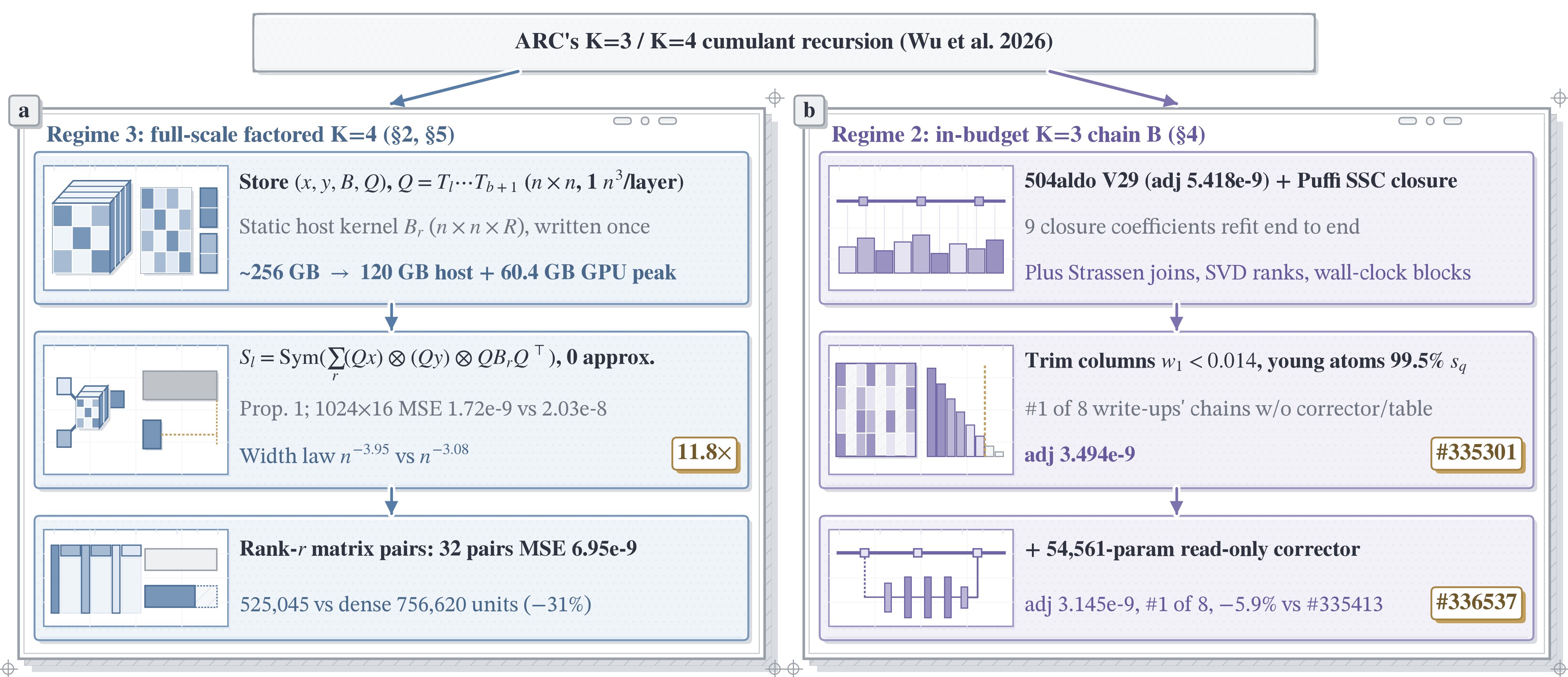
Figure M. Two tracks from ARC’s recursion: factored storage runs exact K=4 at 1024 × 16, 11.8× below augmented K=3; inside the budget, pruning chain B by what later layers read gives #336537, the lowest adjusted error of the eight write-ups, and #335301, first among their chains without a learned corrector or mean-correction table.
Proposition 1 (exact factored source storage). Let a source group born at layer b be Sym(Σ_r x_r ⊗ y_r ⊗ B_r), with birth legs x, y ∈ ℝ^(n×R) and birth kernel slices B_r ∈ ℝ^(n×n), and let every later layer t move each live source by one matrix T_t on all four indices (the linear step and the ReLU carry). Then at every layer l > b, exactly, S_l = Sym(Σ_r Qx_r ⊗ Qy_r ⊗ Q B_r Qᵀ) with Q = T_l T_(l−1) ⋯ T_(b+1). Proof idea: one matrix acts on every index, so T^⊗4 commutes with Sym and maps each product term factor by factor; induction over the layers gives Q (full proof in the PDF, Appendix A.9). Storing (x, y, B, Q) therefore adds no approximation: a group transports one n×n matrix per layer in place of 2n²R numbers. Exact factored storage and transport remove the 256 GB dense transport memory wall with no representation approximation, leaving the n⁴ reads of Q B_r Qᵀ as the target of section 5’s low-rank bilinear compression.
“raw” is the final-layer MSE against ARC’s 10⁹-sample reference; C/B is metered flopscope FLOPs over the 2⁴¹ budget; “adj” is raw × max(0.1, C/B), averaged over networks. One unit is one n × n × n matmul, 2n³ = 2³¹ FLOPs, so B = 1024 units. Chain B is the K=3 chain inside #336537 with its corrector off, graded as #335301 (section 6).
Official public networks 0–4, raw (augmented K=3: ARC’s factorized augmented K=3, the strongest in the reference, run in the reference itself).
| network | K=3 simple | K=3 augmented | K=4 cheap n³ subset | K=4 full | K=3 aug ÷ K=4 full |
|---|---|---|---|---|---|
| 0 | 3.70e-8 | 2.06e-8 | 1.01e-8 | 1.65e-9 | 12.5× |
| 1 | 4.46e-8 | 1.99e-8 | 1.16e-8 | 1.81e-9 | 11.0× |
| 2 | 4.59e-8 | 2.08e-8 | 1.13e-8 | 1.68e-9 | 12.4× |
| 3 | 2.18e-8 | 1.17e-8 | 1.80e-9 | 12.1× | |
| 4 | 1.83e-8 | 1.10e-8 | 1.65e-9 | 11.1× | |
| mean | 4.25e-8 (0–2) | 2.03e-8 | 1.11e-8 | 1.72e-9 | 11.8× |
“K=4 full” is ARC’s factor_k4 with augment off and every source type, and its output equals the basic algorithm’s. Ours is the storage and the n³ forms that make it fit at this width (Figure M, left track); each code path matches ARC’s reference to 1e-15 at n = 40. Each network takes 206–299 s on one 96 GB GPU, peaks at 60.4 GB of GPU memory and keeps 120 GB of births in pinned host memory; run from the input in the compact representation of section 5, its portable subset counts at least 77,930 units per network against the 1,024-unit budget. A second machine reproduces networks 0–3 to three digits.
Full K=4’s 1.72e-9 on the five official networks sits 6.4× below the lowest raw error on the 18 October leaderboard, where every entry ranked 1–50 lies between 1.1e-8 and 2.1e-8 on the board’s 50 networks, the decade of ARC’s augmented K=3 (2.03e-8).
2. The gain grows with n/L, and F29’s cells flip
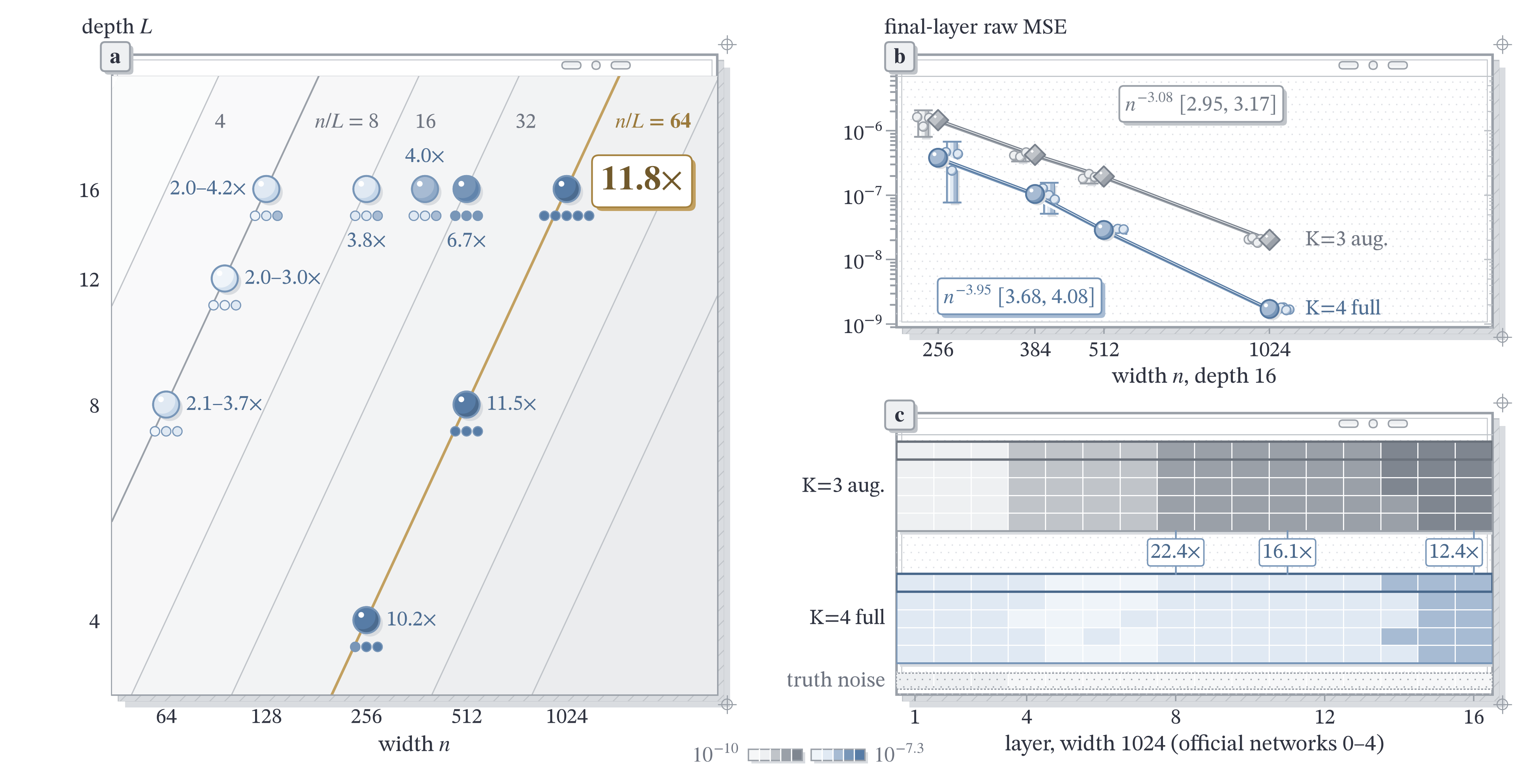
Figure 1. Exact unaugmented K=4 scales as n^−3.95 against augmented K=3’s n^−3.08 and cuts final-layer MSE 11.8× below it at 1024 × 16 on all five official networks; the gain follows n/L, 10.2–11.8× for all three shapes at n/L = 64 and 2.0–4.2× on the nine networks at n/L = 8, the ratio at which F29 found augmented K=4 behind.
(a) Every measured shape on the width × depth plane; diagonals are lines of constant n/L, each station’s label is K=3 aug ÷ K=4 full, dots beneath it are single networks. (b) Raw final MSE against width at depth 16 with fitted exponents. (c) Per-layer MSE of official networks 0–4 at width 1024, with the truth’s sampling noise in the bottom strip.
Width. At depth 16 the 95% network-resample intervals of the two exponents are 3.68–4.08 for full K=4 and 2.95–3.17 for augmented K=3. Each interval holds the exponent, 4 or 3, that the c_K (L/n)^K bound conjectured by Wu et al. (2026, Section 5) gives at fixed depth: the first empirical confirmation of both at the challenge scale, four times the width where the paper’s scan stops (256, its Section 6.3). The measured exponent separation is 0.87 (0.74 to 0.96) at finite depth 16. The ratio is 3.8× at 256, 4.0× at 384, 6.7× at 512 and 11.8× at 1024.
Same n/L, three shapes. At n/L = 64, three new networks at 256 × 4 give 10.2× (8.5–12.3), three at 512 × 8 give 11.5× (10.8–12.1), and the official five at 1024 × 16 give 11.8× (11.3–12.4); holding n/L fixed brings the smaller widths to 0.87 and 0.97 of the challenge value. With the truth noise removed, the ratio grows as (n/L)^p with p = 0.90 (0.77–0.99) across widths and 0.75 (0.55–0.90) across layers 11–16.
Depth. Over layers 8–16, with the truth noise removed, full K=4’s error grows as L^2.9 (2.7 to 3.1 across networks 0–4) and augmented K=3’s as L^2.1, so the ratio narrows from 22.4× at layer 8 to 16.1× at layer 11 and 12.4× at layer 16. The fourth order pays in width and returns part of it in depth, in the direction the L^K of the bound sets.
F29’s cells with unaugmented K=4. 504aldo’s F29 measured augmented K=4 17–20× worse than augmented K=3 at (64, 8) and (96, 12), ran out of memory at (128, 16), and concluded that at n/L = 8 the series is best truncated at K=3. We reran both cells on three new frozen networks each.
| n × L | K=3 aug ÷ K=4 full (unaugmented) | K=4 aug ÷ K=3 aug | F29: K=4 aug ÷ K=3 aug |
|---|---|---|---|
| 64 × 8 | 2.1×, 3.7×, 2.7× | 1.6×, 2.3×, 4.0× | 20× |
| 96 × 12 | 2.5×, 2.0×, 3.0× | past the laptop memory these frozen checks run in | 17× |
| 128 × 16 | 4.2×, 2.0×, 3.2× (earlier order scan) | out of memory |
The augmented variant reproduces F29’s direction, while the unaugmented recursion gains at n/L = 8 on every network. For anyone choosing an order at small n/L: the loss sits in the augmentation, and the fourth order itself pays from n/L = 8 up to 11.8× at n/L = 64.
3. Which state carries the gain
Proposition 2 (readout observability). Let F(s) be the final-layer estimate as a function of a block s of state carried at layer l, every later layer fixed, and g = ∇F(s) its downstream readout vector. For a truncation s − δ, (a) F(s) − F(s − δ) = ⟨g, δ⟩ + O(‖δ‖²), with |⟨g, δ⟩| ≤ ‖g‖ ‖δ‖; (b) the relative readout loss |⟨g, δ⟩| / |⟨g, s⟩| has no bound in terms of the relative norm loss ‖δ‖ / ‖s‖: the norm-optimal rank-one truncation can keep all but a fraction ε of the norm and lose the whole readout. Proof idea: (a) is Taylor and Cauchy–Schwarz; for (b) take s = diag(1, ε) read by g = e₂e₂ᵀ, where Eckart–Young keeps diag(1, 0) and drops exactly what g reads (PDF, Appendix A.9). So we price carried state end to end, by what removing it does to the final error.
Each ReLU layer gives birth to two groups of fourth-cumulant sources, which later layers transport through their weights and ReLU slopes. The two-leg group has three types: star (diagonal kernel 4w₃), path (kernel diag(w₂) C_off diag(w₂)) and C·κ3 (a kernel for every live κ3 source, so it couples the covariance to the whole third cumulant). The slice group holds the (4,), (3,1), (2,2) and (2,1,1) slices that the nonlinearity itself produces; the next layer’s ReLU reads those four slices of κ4, and the (2,1,1) slice also feeds κ3.
Remove one birth type at a time (final MSE ÷ full K=4; frozen columns are networks fixed before running; Monte Carlo truth below 1024):
| removed from full K=4 | 1024 (nets 0–1) | 1024, frozen (nets 5, 6, 7) | 512 | 192 × 16, frozen | 128 × 16, frozen |
|---|---|---|---|---|---|
| nothing: full K=4, raw MSE | 1.73e-9 | 1.42e-9, 1.61e-9, 1.43e-9 | 2.71e-8 | 1.26–2.13e-6 | 1.22–3.13e-5 |
| crossed pairings of the slice births | 1.04 | 1.12, 1.05, 1.05 | 1.04 | 1.09 (1.06–1.13) | 1.09 (1.04–1.15) |
| path births | 1.46 | 1.43, 1.27, 1.51 | 1.26 | 0.98 (0.90–1.13) | 0.92 (0.82–0.97) |
| C·κ3 births | 5.39 | 5.17, 4.67, 5.18 | 2.86 | 2.41 (1.55–3.57) | 0.99 (0.61–1.28) |
| everything except star and same-side slices | 6.28 | 3.65 | |||
| the whole fourth cumulant (= augmented K=3) | 11.7 | 6.64 | 3.37 (2.56–4.81) | 3.12 (2.00–4.17) |
Removing C·κ3 births multiplies final-layer MSE by 0.99× at 128 × 16, 2.41× at 192 × 16, 2.86× at 512 and 5.39× at 1024, where it costs more than every other birth type together, and all three frozen 1024 networks (5, 6 and 7) preserve the full birth-removal ordering C·κ3 > path > slice crossings. Path births pay from 512 up (1.26× at 512, 1.46× at 1024); at 128 and 192, removing them lowers the error on five of six networks, which section 4 explains.
Cut how long sources live (official network 0). Dropping every K=4 source after 2, 3, 4 or 6 layers is 109×, 67×, 41× and 12× worse than keeping all 16, and already worse than K=3 at six layers. Old sources compress where young ones cannot: entering a shared basis of rank 128 after two transports costs 1.29× (3.90e-9 against 3.03e-9 exact), after one transport 1.66×, at birth (rank 112) 3.72×, and at rank 256 after two transports the loss is gone (3.04e-9). For anyone carrying V22’s shared basis to K=4, as we did: let sources enter after their first sensitive reads.
Hand a K=3 chain the K=4 chain’s exact quantities (official networks 0–3, final MSE ÷ augmented K=3). The K=4 chain’s covariance at every layer gives 0.64×, its κ4 alone 0.64×, both together 0.29×, and κ4 only on layers 9–15 along the 64 leading directions of the map to the output 0.81×. The K=4 chain itself reaches 0.08×, 3.6× lower; section 5 runs the same test one level down.
Which reads need exactness. All four output channels close the recursion together: removing one multiplies the error by 1,148 to 714,978. The star crossed pairing pays only exact, and exact costs 3 matmuls. The C·κ3 crossed kernel is close to full rank (rank 16: 1.72×; rank 1: 2.21×). The non-tree term C_jk κ3_ijk, which the factorized K=3 chains of the V29 lineage leave out, is worth 1.56× in our K=4 research chain (4.72e-9 against 3.03e-9, network 0); it is the quickest test for anyone running a V29-lineage chain.
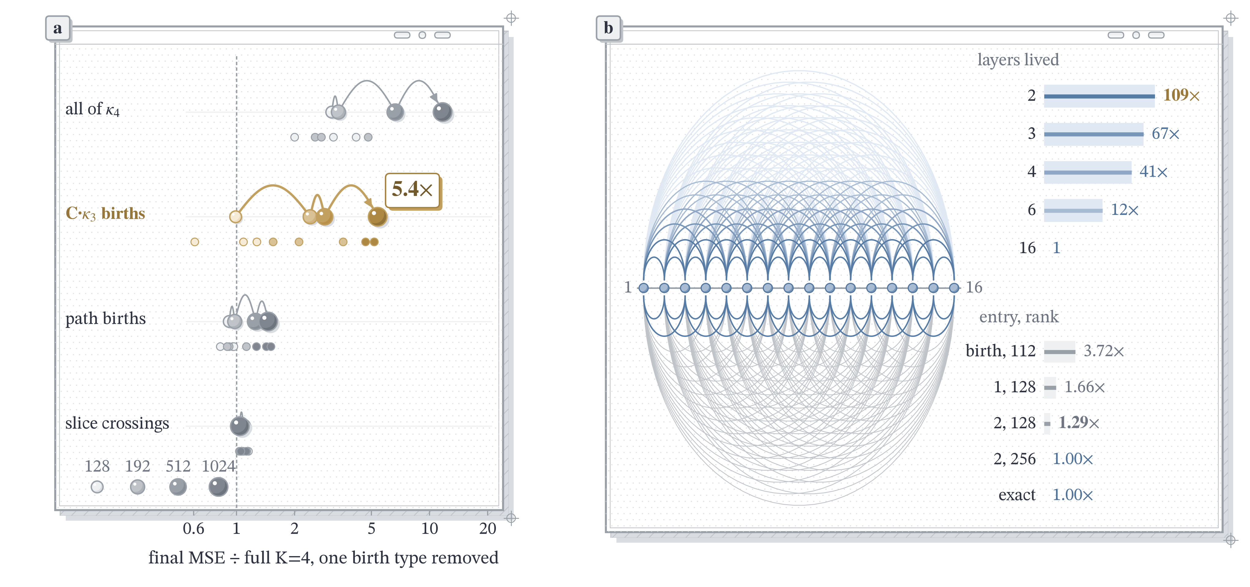
Figure 2. Carried births, not local accuracy, hold the gain: removing C·κ3 births costs 5.4× on official networks 0–1 at width 1024, the largest single removal, and 4.7–5.2× on three networks frozen before running; letting every source live only two layers costs 109×.
(a) One row per birth type removed from full K=4; beads are widths 128, 192, 512 and 1024, small dots single networks frozen before running. (b) The K=4 state of official network 0 drawn as its reads: each arc joins a source’s birth layer to a later layer that reads it. Above the axis, the lifetime ladder; below, reads after a source enters a shared basis, with the cost of each entry age and rank.
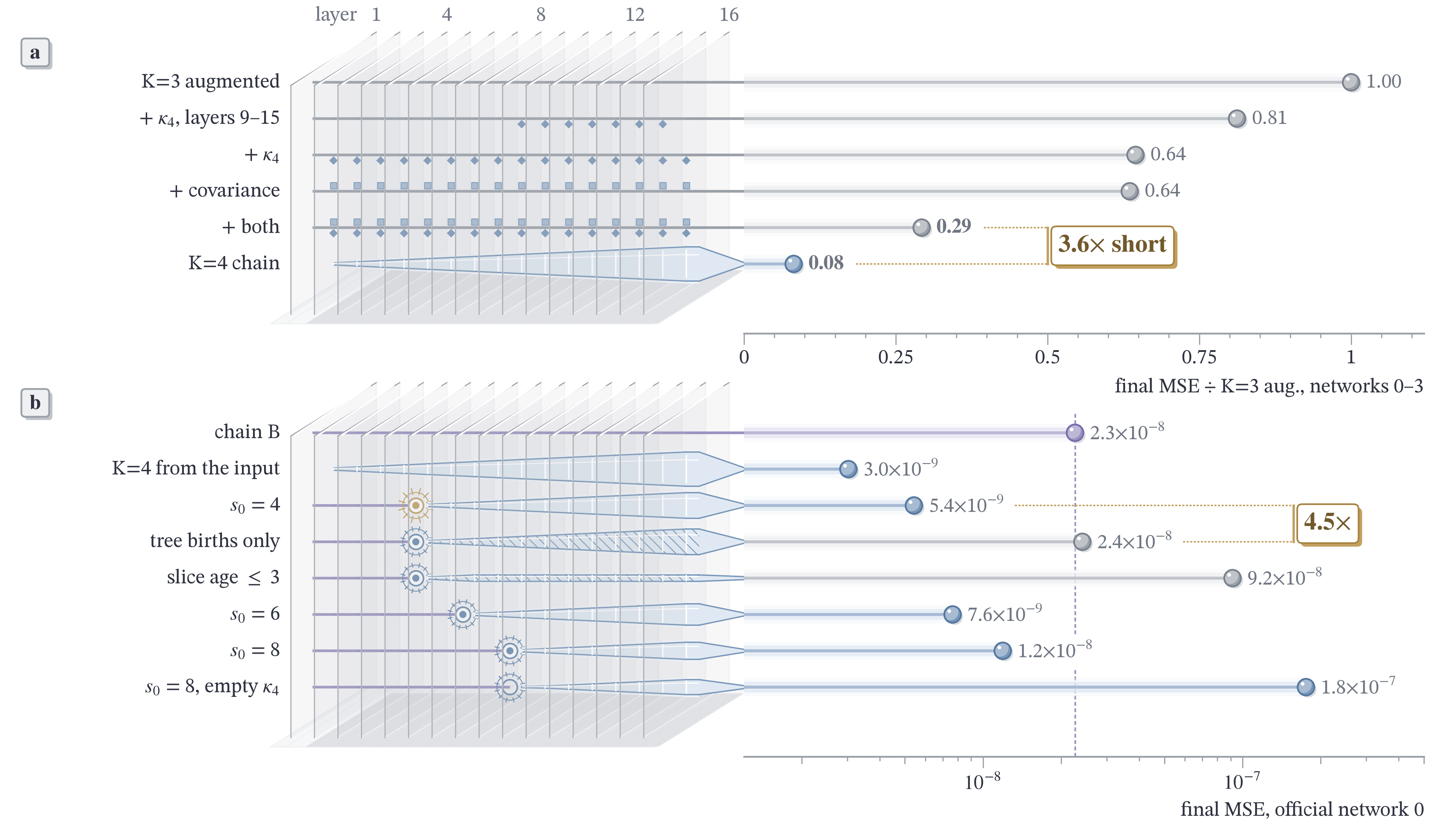
Figure 3. Memoryless patches stall where the carried chain does not: on official networks 0–3, augmented K=3 handed the K=4 chain’s own covariance and κ4 at every layer reaches 0.29 of its error, the K=4 chain 0.08, 3.6× lower; started at layer 4 from chain B, K=4 reaches 5.42e-9, and without its non-tree births it is 4.5× worse.
(a) Ratio to augmented K=3, the exact covariance and κ4 handed in at every layer. (b) Official network 0, chain B alone dashed; the hatched run keeps tree births only and lands back at chain B’s level.
4. Why removing path births helps at small width
Below 1024 the K=4 recursion undercounts star births. On twelve frozen networks (three each at 64 × 8, 96 × 12, 128 × 16 and 192 × 16) we fit the true final-layer means as full K=4 plus reweighted net contributions of path, star and C·κ3 births, each contribution being the full prediction minus the prediction without that type, so weight 1 is the recursion as written. Star weights come out at 1.09–2.04 (median 1.43), above 1 on all twelve, and scaling a network’s star contribution by the mean weight fitted on the other two networks of its shape lowers its final MSE on all twelve, to 0.44–0.97 of full K=4 (geometric mean 0.75). Path births point away from the missing star content: cos(path, star) < 0 exactly where removing path births helps, on 10 of 12 networks and all nine at widths 64–128.
At 1024 the undercount closes: on frozen networks 5, 6 and 7, fitted star weights are 1.03–1.07, leave-one-out star scaling gives 0.994–0.998 of full K=4, path and star births are nearly orthogonal with cos(path, star) from −0.09 to −0.03, and removing star births costs 1.79–2.05× (fitting all three weights in sample moves the final MSE only to 0.91–0.95 of full K=4). Whatever error remains at 1024 lies outside a per-type reweighting.
5. The road to 2⁴¹: two births and one representation
Above 1,024 units a network scores as an all-zero prediction, so full K=4’s accuracy counts once its cost fits. The arithmetic sets the prize: raw 1.72e-9 at C/B 0.75 ties rank 1 of the 18 October board (adj 1.3e-9). The nearer bar is our own. On official network 0 the complete chain from layer 4, at its compressed accuracy of 6.38e-9, beats chain B’s score below 602 units.
The gain does not come in cheap pieces. We added K=4 pieces that fit in 1,024 units to chain B, alone and combined, in 71 settings, read at the output or fed into chain B’s nonlinear moments. Every coefficient comes from the cumulant algebra; ages and ranks were chosen on network 0, then frozen and retested on eight further networks. Where they help they buy 0.9–1.8% raw, with the sign set network by network. The best, star births with the (4,) and (3,1) slices fed back, gives −1.8% on the eight frozen networks (95% t interval −3.6% to +0.03%) at 976 units, which puts adj at 5.6× chain B’s. The 11.8× needs full-rank C·κ3 crossings, non-tree births and long-lived slice groups together.
Started late, K=4 keeps most of the gain, through non-tree births. On official network 0, chain B alone gives 2.26e-8. Running chain B to layer 4 and the portable K=4 set from there (full K=4 without path births and slice crossings), seeded from chain B’s own κ4 slices, gives 5.42e-9. Tree-type births alone give 2.41e-8, 1.07× of chain B, so the non-tree births carry the whole late-start gain. Without C·κ3 births the late start lands at 1.13e-8, 2.1× worse.
What the complete chain costs (counted lower bound, compact legs-and-kernels representation, network 0):
| from layer | counted units | C·κ3 + non-tree share | raw, compressed as counted | units to tie chain B’s adj |
|---|---|---|---|---|
| 0 | 77,930 | 95% | 4.33e-9 | 888 |
| 4 | 60,549 | 96% | 6.38e-9 | 602 |
| 6 | 47,287 | 96% | (exact 7.64e-9) | ≤503 |
| 8 | 33,611 | 96% | (exact 1.19e-8) | ≤322 |
Units and gain sit in the same two families (from layer 4; read weight defined below; “without ÷ with”: final MSE without the family over with it; last column full K=4 from the input unless a cell names the portable set or networks 5–7):
| state family | units | share | first-order read weight | without ÷ with, from layer 4 | without ÷ with, from the input |
|---|---|---|---|---|---|
| C·κ3 births | 27,390 | 45.2% | 33.2% | 2.08 | 5.39 (frozen 5.17, 4.67, 5.18) |
| non-tree births | 30,705 | 50.7% | 6.4% | 1.95 | 1.56 for C_jk κ3_ijk alone, portable set |
| tree slices + (2,1,1) → K3 feedback | 1,814 | 3.0% | 30.3% | alone, 1.07× worse than chain B | slice crossings 1.04 |
| star births, K=4 sources, young legs | 473 | 0.8% | 30.2% | 1.10 (C·κ3 off) | 1.79–2.05 (frozen 5–7) |
| chain B, metered | 168 | 0.3% |
The cost sits where the gain sits. A C·κ3 birth at layer b carries 9,216·b columns of κ3 legs, so each (birth, read) pair costs 63b units and the row grows cubically in depth; a non-tree birth’s first read costs 3,070.5 units. Everything outside the two families sums to 2,454 units, 2.4 budgets, and does not beat chain B on its own (tree slices 1.07×, with star births 2.87×).
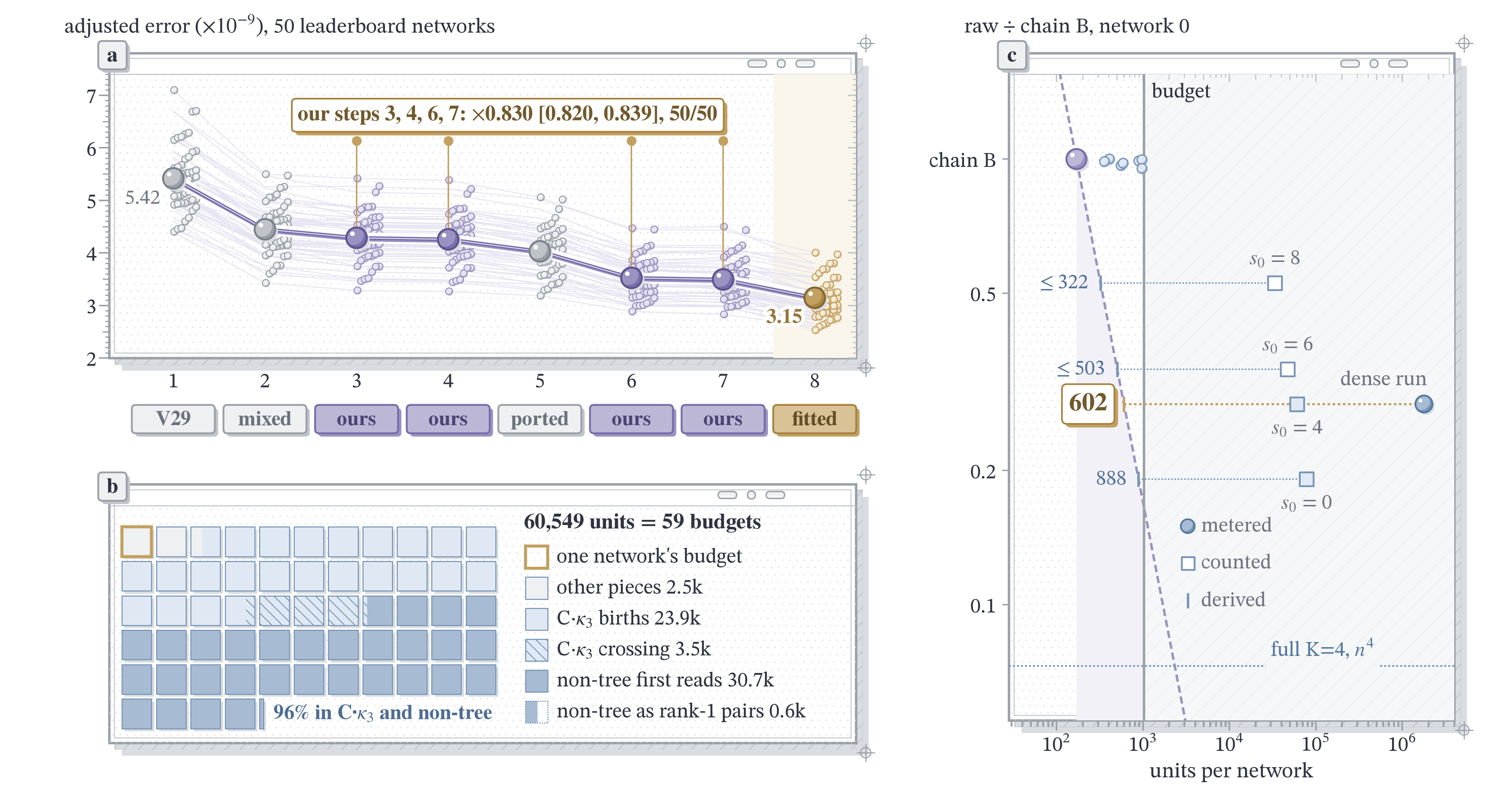
Figure 4. Our own steps multiply the grader’s mean adjusted error by 0.830 [0.820, 0.839], lower on all 50 leaderboard networks; the complete K=4 chain from layer 4, counted at 60,549 units, ties chain B’s score at 602.
(a) The eight grader receipts of section 6; each thin line is one of the 50 leaderboard networks, the tags give the origin of each step. (b) The complete chain from layer 4 as tiles of one network’s budget, 96% in C·κ3 and non-tree births. (c) Cost against accuracy on network 0; the dashed diagonal is chain B’s score, and each counted configuration ends at the units where it ties chain B.
Local rulers point away from the gain. Three ways of choosing what to keep, each against chain B, every raw recomputed from its saved prediction.
Exact local content. We put the object of kai_leal_gonzalez’s 18246, the exact (3,1) slice of κ4 (public 10⁸-sample pair moments, layers 1–14), into chain B without its corrector. It gives 0.873 of chain B’s raw over eight mini networks, 7 of 8 lower, in line with 18246’s −18.1% inside V29. On networks 0, 1, 3 and 4, where full K=4 also ran, that is 10.0%, −0.2%, 8.2% and 3.5% of the K=4 log gain; the K=4 chain’s own births hold the rest.
A first-order read weight. Score every counted (state, read) pair by the first-order effect of its read on the final mean, through the next layer’s mean and variance (or also through κ3). Non-tree births get 6.4% of the weight and carry 1.95×. Keeping reads in order of that weight is 3.4–22× worse than chain B at every size we measured from 600 to 20,452 units, on both networks (11 configurations), while the reverse order at 20,451 units gives 0.703×. Local fidelity is not downstream value, the split jamesrahenry’s Phase 1 carrier showed for the third cumulant (section 8).
Deleting state. The best deletion rule keeps whole lives and a consistent state: tree slices born at every layer, non-tree and star births born early. It reaches 0.937× of chain B’s raw at 8,194 units, 0.833× at 11,296 and 0.615× at 20,586 (network 1: 0.910× and 0.703×); without the late tree slices the same window is 1.80× worse than chain B. Chain B’s score prices each point. At 0.615× a network may spend 276 units to tie it, and the rule spends 75× that (45× at 0.937×), 18,423 of its 20,586 units in the dense first reads of six non-tree births.
Compressing the births moves the envelope. The non-tree term does not self-average: over the current layer’s weights its mean is exactly zero at the first read, and over older sources it carries 1.5–3.7% of the readout energy in two of the four channels and none in the other two. At n = 64 a covariance Krylov basis keeps none of its gain and a Rademacher sketch keeps 40% at rank 1 and 92% at rank 16, while matrix pairs along the kernel’s own direction, from unfolding the birth kernel on its repeated index, keep 79–84% at rank 1 on three networks and 101% at rank 2. We took that form to n = 1024 (network 0, counted in the same representation, real κ3 leg width kept) and held the six non-tree births of the 20,586-unit rule as pairs:
| births kept, held as pairs at rank | units | raw ÷ chain B | units ÷ tie | deletion needs, units |
|---|---|---|---|---|
| the 20,586-unit rule, dense | 20,586 | 0.615 | 75× | |
| the same births, non-tree rank 16 | 6,321 | 0.681 | 25× | 17,492 |
| the same births, non-tree rank 4 | 3,258 | 0.788 | 15× | 14,396 |
| the same births, non-tree rank 1 | 2,493 | 0.942 | 14× | 8,194 |
| births at 4–13, both families rank 8 | 33,215 (9,345 + 23,870 κ3 legs) | 0.555 | 109× | 32,687 |
“Deletion needs” is the cheapest deletion point with no higher raw. At rank 4 that point is 14,396 units at 0.749×, so the pairs need 77% fewer units, and all three non-tree points join the lower envelope. The six non-tree births cost 330, 1,095 and 4,159 units at ranks 1, 4 and 16, against 18,423 dense. Compressing both families shows where the next cut lies: as pairs, the C·κ3 births still pay 23,870 units of κ3 leg width, 63b units per (birth, read) pair.
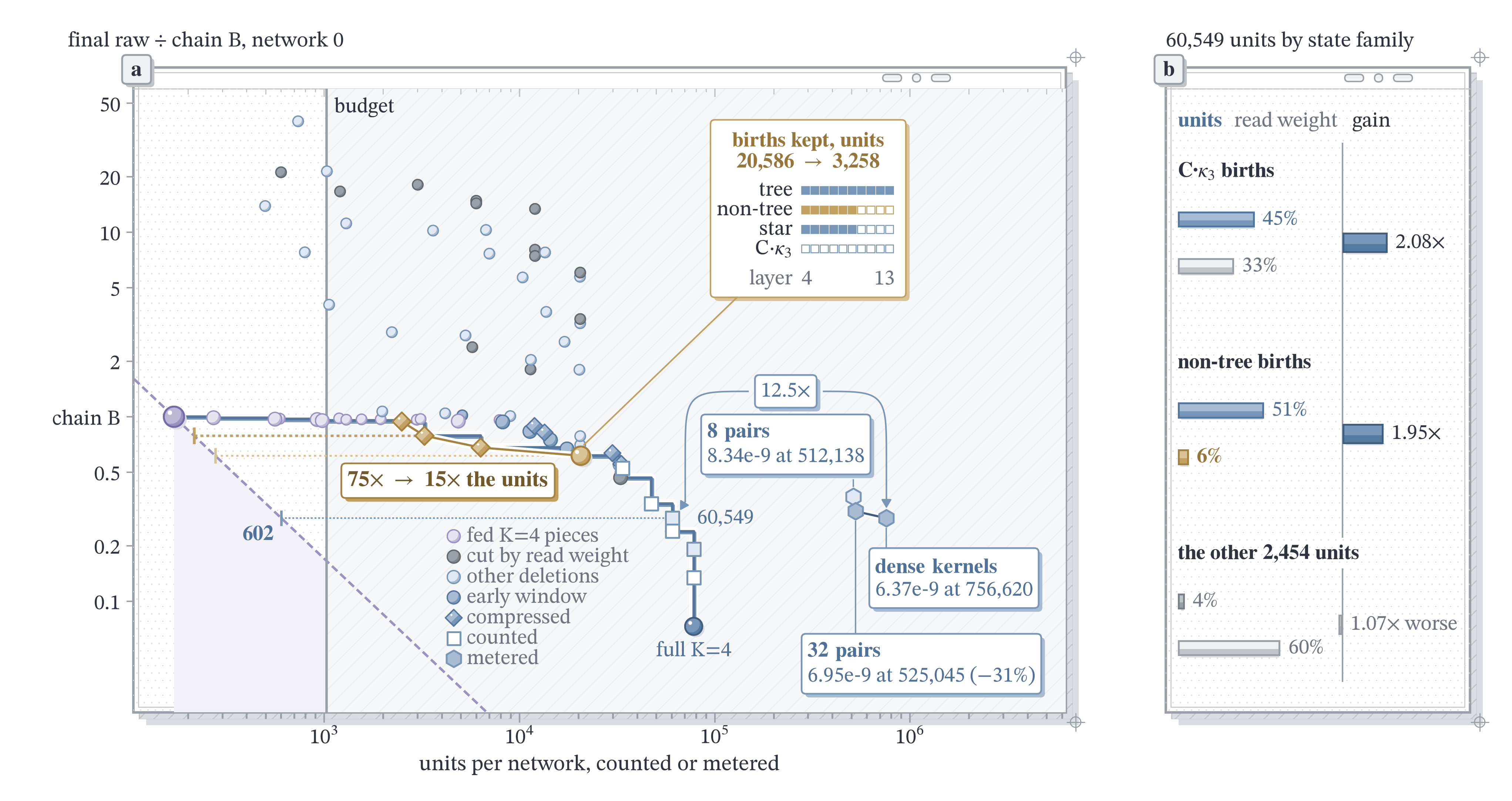
Figure 5. One compute–error frontier on official network 0, inside the budget and beyond it: deleting state stalls at 75 times the units its accuracy may cost (0.615× of chain B’s error at 20,586 units), rank-4 non-tree pairs cut that to 15 times (0.788× at 3,258), and the metered whole chain falls from 756,620 units with dense kernels to 525,045 with 32 matrix pairs at 6.95e-9.
(a) Final raw over chain B’s against units; the stair is the lower envelope, the dashed diagonal chain B’s score. Gold: the best deletion rule (tie at 276) and, along the gold line, the same births with non-tree pairs of rank 16, 4 and 1 (rank 4 ties at 215); blue diamonds compress both families; squares are counted; hexagons are metered end to end by flopscope, each named in a capsule, and the arc marks the 12.5× between the counted chain (60,549 units) and the dense metered run at one raw. (b) The layer-4 chain by family: share of the units, share of the first-order read weight, and the gain each family carries.
Metered end to end. We ran the whole compressed chain from layer 4 on official network 0 with every operation executed and billed by flopscope 0.12.3: old sources in one k = 128 core, old feedback in a k₃ = 128 core, the (2,2) and (2,1,1) slice kernels dense, every birth kept for life. Accuracy holds: final raw 6.37e-9 against the 6.38e-9 the ledger counts, each layer within 0.14% of the GPU research chain. The meter reads 756,620 units (C/B 739), 12.5× the counted lower bound. One network takes 6.2 h and 114.8 GiB on a CPU host; official network 1 is traced through layer 14 at 6.48e-9.
| ledger rows, from layer 4 | counted | metered |
|---|---|---|
| C·κ3 and star births, sources, young legs | 27,863 | 193,000 |
| old slice reads (tree) | 1,430 | 135,961 |
| non-tree first reads | 30,705 | 345,045 |
| old feedback | 384 | 33,724 |
| chain B to layer 4 | 168 | 25 |
| outside the count (κ3 expanded dense, linear steps) | 48,864 | |
| total (rows rounded) | 60,549 | 756,620 |
Most of the excess has one source. 88% of the metered units are reads of the slice and two-leg groups, each an n⁴ product because κ3 is stored dense, so every (2,1,1) feedback lands as an n³ tensor; the ledger counts the same reads with κ3 and the feedback in factors. The two rows that hold the two families bill 538,045 units, 71%. Holding the (2,1,1) birth kernel as 8 matrix pairs takes the meter to 512,138 units (the pairs cost 2,133 against 30,705 dense) at raw 8.34e-9. With 32 pairs, run through all 16 layers, the chain holds 6.95e-9 at 525,045 units: 30.6% fewer units than the dense kernels for 9.1% more raw, and 872× the 602-unit target where the dense run stands at 1,257×. Compressing the whole kernel compresses its tree terms too, where the pairs in the table above compress the non-tree part alone; with 32 pairs, 87% of the units are still reads a dense κ3 forces.
The next cut. The family split, the first compression and the meter point at one place, κ3’s representation: a dense old part plus young factors, with the (2,1,1) feedback written into the young factors in place of an n³ tensor, the form in which the ledger counts these reads at 63b units a pair. C·κ3 births then need legs built at low rank before the birth, toward the 3 matmuls of the star crossing, and the other 2,454 units need a shared core for old slice groups that keeps the channels an energy basis loses (section 7, row 17). ARC calls random networks the base case of an induction toward trained models. At the challenge shape that base case now has its fourth order measured, its value located in two births, and its remaining price traced to one representation.
Continued in the next post: the scored chain (section 6), twenty falsified closure hypotheses (section 7), the other public write-ups on the same grader (section 8), how to reproduce every number (section 9) and the three structural laws with our position (section 10).