Sharing this notebook so that more people can get a headstart on how to use pre-trained models to get better results.
![]()
FOODC Resnet50 submission
This notebook basically follows the baseline notebook and instead of training a network from scratch we use Resnet 50 model and train it for 25 epochs.
Author - Pulkit Gera
To open this notebook on Google Computing platform Colab, click below!
![]()
Download the files
These include the train test images as well the csv indexing them
!wget -q https://s3.eu-central-1.wasabisys.com/aicrowd-practice-challenges/public/foodc/v0.1/train_images.zip
!wget -q https://s3.eu-central-1.wasabisys.com/aicrowd-practice-challenges/public/foodc/v0.1/test_images.zip
!wget -q https://s3.eu-central-1.wasabisys.com/aicrowd-practice-challenges/public/foodc/v0.1/train.csv
!wget -q https://s3.eu-central-1.wasabisys.com/aicrowd-practice-challenges/public/foodc/v0.1/test.csv
We create directories and unzip the images
!mkdir data
!mkdir data/test
!mkdir data/train
!unzip train_images -d data/train
!unzip test_images -d data/test
Import necessary packages
import torchvision.transforms as transforms
from torch.utils.data.sampler import SubsetRandomSampler
import torch
import torch.nn as nn
import torch.nn.functional as F
from torch.optim import lr_scheduler
from torch.utils.data import TensorDataset, DataLoader, Dataset
import torchvision
from torchvision import models
import torch.optim as optim
import pandas as pd
import numpy as np
import cv2
import os
from sklearn import preprocessing
import matplotlib.pyplot as plt
%matplotlib inline
import time
Loading Data
In pytorch we can directly load our files into torchvision(the library which creates the object) or create a custom class to load data. The class must have __init__ , __len__ and __getitem__ functions. We create a custom dataloader to suit our needs. More info on custom loaders can be read here
class FoodData(Dataset):
    def __init__(self,data_list,data_dir = './',transform=None,train=True):
        super().__init__()
        self.data_list = data_list
        self.data_dir = data_dir
        self.transform = transform
        self.train = train

    def __len__(self):
        return self.data_list.shape[0]

    def __getitem__(self,item):
        if self.train:
          img_name,label = self.data_list.iloc[item]
        else:
          img_name = self.data_list.iloc[item]['ImageId']
        img_path = os.path.join(self.data_dir,img_name)
        img = cv2.imread(img_path,1)
        img = cv2.resize(img,(256,256))
        if self.transform is not None:
            img = self.transform(img)
        if self.train:
          return {
              'gt' : img,
              'label' : torch.tensor(label)

          }
        else:
          return {
              'gt':img
          }
We first convert the data labels into encodings using Label Encoders. This basically converts labels into number encodings. This is an important step as without it we cannot train our network
train = pd.read_csv('train.csv')
le = preprocessing.LabelEncoder()
targets = le.fit_transform(train['ClassName'])
ntrain = train
ntrain['ClassName'] = targets
We load our train data and some necessary augementations like converting to PIL image, converting to tensors and normalizing them across channels. We can add more augementations such as Random Flip, Random Rotation, etc more on which can be found here. Augmentation is an important step and helps increasing the data size. The more data the better the model.
transforms_train = transforms.Compose([
    transforms.ToPILImage(),
    transforms.RandomRotation(90),
    transforms.RandomHorizontalFlip(),
    transforms.ColorJitter(),
    transforms.ToTensor(),
    transforms.Normalize( mean = np.array([0.485, 0.456, 0.406]),
    std = np.array([0.229, 0.224, 0.225]))
])
train_path = 'data/train/train_images'
train_data = FoodData(data_list= ntrain,data_dir = train_path,transform = transforms_train)
EDA
Let us do some exploratory data analysis. The idea is to see the class distribution, how the images are and much more.
train = pd.read_csv('train.csv')
num = train['ClassName'].value_counts()
classes = train['ClassName'].unique()
print("Percentage of each class")
for cl in classes:
  print(cl,'\t',num[cl]/train.shape[0]*100,"%")
We observe that water is the most popular class although the distribution is not that skewed. Let us plot the images of white flour french bread and french fries and have a look at the kind of images we have
imgs = train.loc[train['ClassName'] == 'bread-french-white-flour']
plt.figure(figsize=(10,10))
for i in range(imgs[:16].shape[0]):
  path = imgs.iloc[i]['ImageId']
  image = cv2.imread(os.path.join(train_path,path),1)
  image = cv2.cvtColor(image,cv2.COLOR_BGR2RGB)
  plt.subplot(4,4,i+1)
  plt.axis('off')
  plt.imshow(image)
imgs = train.loc[train['ClassName'] == 'chips-french-fries']
plt.figure(figsize=(10,10))
for i in range(imgs[:16].shape[0]):
  path = imgs.iloc[i]['ImageId']
  image = cv2.imread(os.path.join(train_path,path),1)
  image = cv2.cvtColor(image,cv2.COLOR_BGR2RGB)
  plt.subplot(4,4,i+1)
  plt.axis('off')
  plt.imshow(image)
Split Data into Train and Validation
Now we want to see how well our model is performing, but we dont have the test data labels with us to check. What do we do ? So we split our dataset into train and validation. The idea is that we test our classifier on validation set in order to get an idea of how well our classifier works. This way we can also ensure that we dont overfit on the train dataset. There are many ways to do validation like k-fold,leave one out, etc
We also make dataloaders which basically create minibatches of dataset which are used in each epoch
Although the data is not that imbalanced, one idea we can add is SMOTE which helps in sampling incase of imbalanced classification where it samples multiple times. I havent tried that but it works well. Read more about it here
batch = 64
valid_size = 0.2
num = train_data.__len__()
# Dividing the indices for train and cross validation
indices = list(range(num))
np.random.shuffle(indices)
split = int(np.floor(valid_size*num))
train_idx,valid_idx = indices[split:], indices[:split]

#Create Samplers
train_sampler = SubsetRandomSampler(train_idx)
valid_sampler = SubsetRandomSampler(valid_idx)

train_loader = DataLoader(train_data, batch_size = batch, sampler = train_sampler)
valid_loader = DataLoader(train_data, batch_size = batch, sampler = valid_sampler)
Here we load test images. Note: This file will not have any labels with it
transforms_test = transforms.Compose([
    transforms.ToPILImage(),
    transforms.ToTensor(),
    transforms.Normalize( mean = np.array([0.485, 0.456, 0.406]),
    std = np.array([0.229, 0.224, 0.225]))
])
test_path = 'data/test/test_images'
test = pd.read_csv('test.csv')
test_data = FoodData(data_list= test,data_dir = test_path,transform = transforms_test,train=False)

test_loader = DataLoader(test_data, batch_size=batch, shuffle=False)
Here we check if we have a GPU or not. If we have we just need to shift our data and model to GPU for faster computations.
device = torch.device("cuda:0" if torch.cuda.is_available() else "cpu")

# Assuming that we are on a CUDA machine, this should print a CUDA device:

print(device)
Define the Model
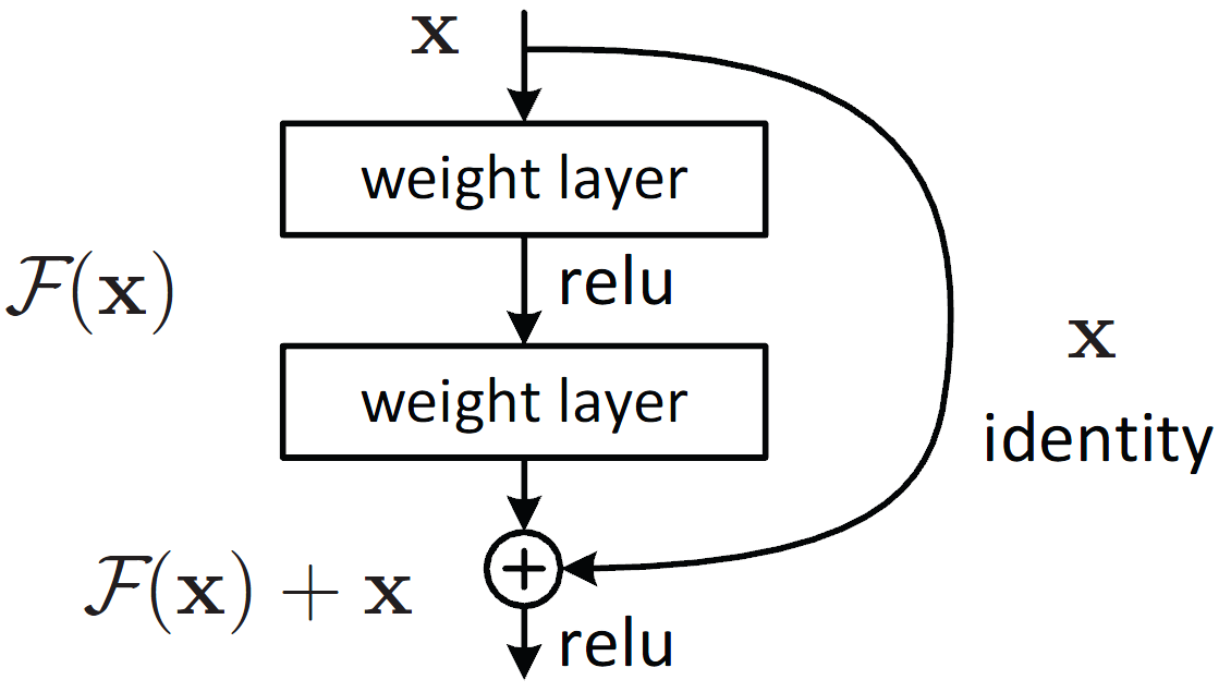
We are going to use ResNet50. The idea was born from the fact that deeper the models are , after a certain point their accuracy becomes poor. This is due to the fact that gradients passed back become smaller and smaller which leads to negligible change in the early layers.
In order to combat that, we add skip connections to layers forward. This way we are able to preserve the gradients and build deeper models.
Pytorch provides a collection of pretrained resnet architectures. We use resnet 50.
To read more about resnet and its variants, this is a good blog
More on pretrained models with pytorch here and making models here.
train_sampler.__len__()
dataloaders = {}
dataset_sizes = {}
dataloaders['train'] = train_loader
dataloaders['val'] = valid_loader
dataset_sizes['train'] = train_sampler.__len__()
dataset_sizes['val'] = valid_sampler.__len__()
Train
Alright enough talk and time to train. We define the number of epochs and train the model. An epoch is a forward pass and backward pass of all the data points. An epoch consists of iterations which depend on batch size. So basically we take a batch, get its output, do a backward pass and let the optimizer take a step. This is the workflow for any pytorch code.
Validate
Now after an epoch ends, we check with validation and do the same steps except backward pass on loss and optimizer step. If we get a reduction in validation loss, we save the model. This is sort of an early stopping.
def train_model(model, criterion, optimizer, scheduler, num_epochs=25):
    since = time.time()

    best_model_wts = copy.deepcopy(model.state_dict())
    best_acc = 0.0

    for epoch in range(num_epochs):
        print('Epoch {}/{}'.format(epoch, num_epochs - 1))
        print('-' * 10)

        # Each epoch has a training and validation phase
        for phase in ['train', 'val']:
            if phase == 'train':
                model.train()  # Set model to training mode
            else:
                model.eval()   # Set model to evaluate mode

            running_loss = 0.0
            running_corrects = 0

            # Iterate over data.
            for data in dataloaders[phase]:
                inputs = data['gt'].squeeze(0).to(device)
                labels = data['label'].to(device)
                # inputs = inputs.to(device)
                # labels = labels.to(device)

                # zero the parameter gradients
                optimizer.zero_grad()

                # forward
                # track history if only in train
                with torch.set_grad_enabled(phase == 'train'):
                    outputs = model(inputs)
                    _, preds = torch.max(outputs, 1)
                    loss = criterion(outputs, labels)

                    # backward + optimize only if in training phase
                    if phase == 'train':
                        loss.backward()
                        optimizer.step()

                # statistics
                running_loss += loss.item() * inputs.size(0)
                running_corrects += torch.sum(preds == labels.data)
            if phase == 'train':
                scheduler.step()

            epoch_loss = running_loss / dataset_sizes[phase]
            epoch_acc = running_corrects.double() / dataset_sizes[phase]

            print('{} Loss: {:.4f} Acc: {:.4f}'.format(
                phase, epoch_loss, epoch_acc))

            # deep copy the model
            if phase == 'val' and epoch_acc > best_acc:
                best_acc = epoch_acc
                best_model_wts = copy.deepcopy(model.state_dict())

        print()

    time_elapsed = time.time() - since
    print('Training complete in {:.0f}m {:.0f}s'.format(
        time_elapsed // 60, time_elapsed % 60))
    print('Best val Acc: {:4f}'.format(best_acc))

    # load best model weights
    model.load_state_dict(best_model_wts)
    return model
import copy
model_ft = models.resnet50(pretrained=True)
# To only train the last layer
# for param in model_ft.parameters():
#     param.requires_grad = False
num_ftrs = model_ft.fc.in_features

# Alternatively, it can be generalized to nn.Linear(num_ftrs, len(class_names)).
model_ft.fc = nn.Linear(num_ftrs, 61)

model_ft = model_ft.to(device)

criterion = nn.CrossEntropyLoss()

# Observe that all parameters are being optimized
optimizer_ft = optim.Adam(model_ft.parameters(), lr=0.001)

# Decay LR by a factor of 0.1 every 7 epochs
exp_lr_scheduler = lr_scheduler.StepLR(optimizer_ft, step_size=7, gamma=0.1)
Here we define our model object along with our optimizer and error function. Typically for multi class classification we use Cross Entropy Loss. More about different types of losses are here.
We use the popular Adam optimizer with its default parameters. There are other optimizers like SGD, RMSPROP, Adamax,etc. You can have a detailed look at optimizers here
You must be wondering what is a scheduler. A scheduler provides a policy for the decay of learning rate. For example we can say that let the learning rate value decrease after some fixed number of epochs or say if the validation accuracy doesnt change, we can change the learning rate. This helps in faster and better convergence. Read more here
model_ft = train_model(model_ft, criterion, optimizer_ft, exp_lr_scheduler,
                       num_epochs=25)
Predict on Validation
Now we predict our trained model on the validation set and evaluate our model
# model.load_state_dict(torch.load('best_model_so_far.pth'))
model_ft.eval()
correct = 0
total = 0
pred_list = []
correct_list = []
with torch.no_grad():
    for images in valid_loader:
        data = images['gt'].squeeze(0).to(device)
        target = images['label'].to(device)
        outputs = model_ft(data)
        _, predicted = torch.max(outputs.data, 1)
        total += target.size(0)
        pr = predicted.detach().cpu().numpy()
        for i in pr:
          pred_list.append(i)
        tg = target.detach().cpu().numpy()
        for i in tg:
          correct_list.append(i)
        correct += (predicted == target).sum().item()

print('Accuracy of the network on the 10000 test images: %f %%' % (
    100 * correct / total))
from sklearn.metrics import f1_score,precision_score,log_loss
print("F1 score :",f1_score(correct_list,pred_list,average='micro')*100)
Predict on test set
Time for the moment of truth! Predict on test set and time to make the submission.
# model.load_state_dict(torch.load('best_model_so_far.pth'))
model_ft.eval()

preds = []
with torch.no_grad():
    for images in test_loader:
        data = images['gt'].squeeze(0).to(device)
        outputs = model_ft(data)
        _, predicted = torch.max(outputs.data, 1)
        pr = predicted.detach().cpu().numpy()
        for i in pr:
          preds.append(i)
Save it in correct format
# Create Submission file
df = pd.DataFrame(le.inverse_transform(preds),columns=['ClassName'])
df.to_csv('submission.csv',index=False)
To download the generated in collab csv run the below command
from google.colab import files
files.download('submission.csv')