Hi everyone,
I create this thread to discus the loading strategies and price sensitivity studies you ran during the game.
@simon_coulombe described his attempt to create random shock on his margin (but didn’t receive enough feedback to leverage it ). I also hoped @alfarzan would give us this feedback (would have opened many possibilities) but it would have created unfair information for those who joined the competition early…
On my side I tried the following strategy :
I took a variable which was not very relevant (vehicle fuel) and well balanced. I guessed everybody would capture its effect correctly :
On week 8, I used the “fair price” to both types of fuels, and confirmed my underwriting results followed the train data distribution.
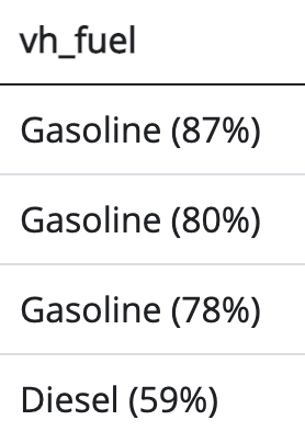
On week 9, I gave a 10% price increase to the diesel vehicles (keeping gaz untouched). In the weekly feedback I got a very strong difference in the underwriting results.
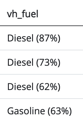
To be sure, I did the same on week 10 (this time decreasing diesel, still leaving the gaz at the same price).
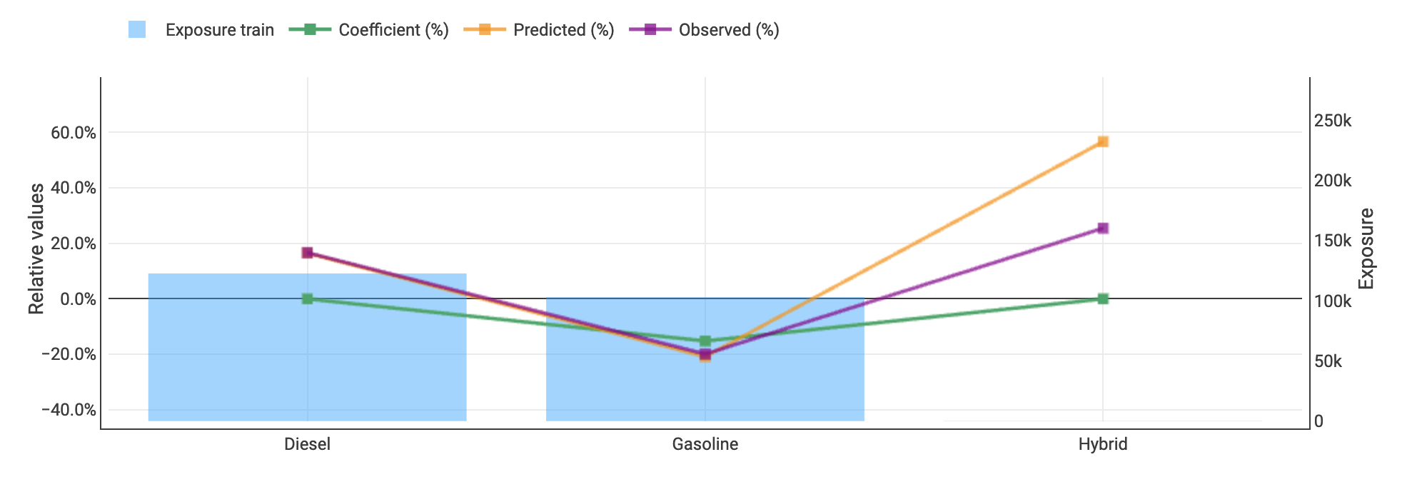
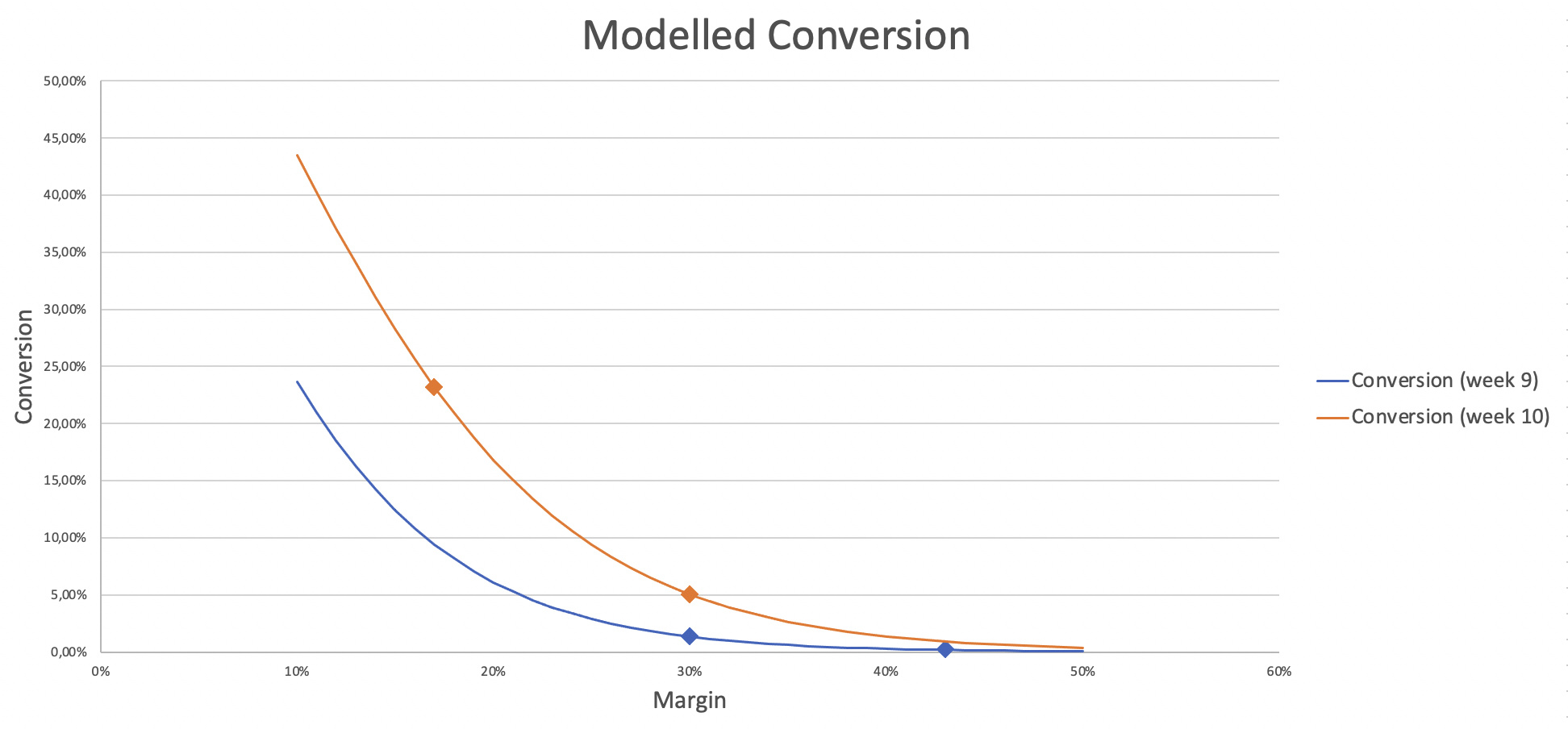
Finally I used these results (combined with the size of each conversion levels, the average conversion in each level, and the number of vehicles in each category) to estimate the conversion rate for each vehicle and, then, the impact on the 10% increase or decrease on the conversion. So I could finally build a conversion model for each round :
the elasticity of our markets are very large (above 15) which makes sense in a winner takes all environment
the market shifted by about 7% between weeks 9 and 10, which led to very different conversion results at the same price. This instability creates a huge element of luck in the results (this is coherent with what we saw on the leaderboard, with some ranks changing dramatically while the submissions were not edited).
@alfarzan has the real data to compute this kind of curves, and it would be interesting to know what they really look like - my computation is full of ugly approximations !!!
Did anyone else try to estimate these elements of the market ?
Some very interesting work you’ve done! Can you please share the R code you used to create the first relativity graph in your post? (The one with the vehicle fuel relativity, I’d like to try reproduce it).
I decided to try something quite different, I started investigating utility curves for the insurer and insured. It is possible to find a maximum premium that the insured is prepared to accept and a minimum premium the insurer is prepared to charge by using utility curves. Diminishing marginal utility would suggest a logarithmic curve for the insured. The calculations I produced gave a premium of 1115! Very large compared to the risk premium calculations (including loadings etc.), could be the initial wealth estimates.
not gonna lie, using the fuel type variable to calculate price elasticity given our constraints is pretty cool.
Now I wonder if there were any other variables you could have used to get more than 2 points per week.
I’ll need to dig out exactly what I did, but I think I came up with an elasticity at 0 of around 20-25 in a vacuum. (so this gives me an idea of the underlying elasticity that exists from the nature of the comp with 10 equivalent competitors, but is probably inferior to your direct market probing) I think I generated a market of 10 competitors using the same lgb model built with 10 different seeds, and then playing around with the load/discount applied to individual competitors etc.
That’s a very interesting approach to estimating elasticity.
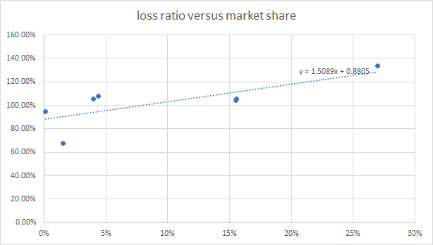
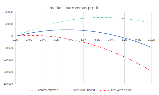
I only applied a more broad brush approach by fitting lines to graphs of market shares and profit results from different weeks, and estimating potential profits at different market shares. This was done by multiplying market share by an assumed average premium by 100% minus the expected loss ratio from the fitted line. I tried fitting a few different lines by making various heroic assumptions about how the market might have moved from week to week based on very little data and concluded my model needed market share somewhere around 4 to 5% to make the most profit. I also looked at the past loadings I applied and what they achieved in terms of market share and made a rough guess of what I need to do to get a market share of roughly 4.5%. I have no idea if everyone suddenly decided to change prices significantly for the final submission – in which case my estimates could be out wildly.
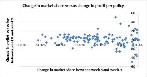
I attempted to estimate the potential variability of the result, and it is huge. In order to estimate the potential variability of results I looked at how profitability changed from week to week for people who didn’t submit a change in model. Between week 8 and week 9 it looks like the variability in profit per policy from week to week was within a range of +/- 20. The graph below shows changes in profit per policy for all people with unchanged models between week 8 and week 9 versus their change in market share (profit per policy was estimated by estimating the average number of polices each person wrote as being their market share multiplied by an assumed 30,000 policies each week, I then divide weekly profit from the leader board by their estimated number of policies):
The variability in profit per policy between week 9 and week 10 was similar for people who didn’t submit a model change, so I assumed +/-20 is a reasonable estimate for the variability in profit margin when there are 30,000 policies. The final dataset is three times bigger, and assuming the variability in profit reduces in line with the square root of the number of policies gives a guess of about +/-12 in the variability of the potential profit per policy for the final submission. I concluded that my loss ratio is likely to end up in the range 85%-105%. It all depends on which policies end up having large claims.
As you guess, the results of this study were a bit useless:
the market is moving too quickly to leverage the results ; the results are true for one week, but the market will have shifted for the following leaderboard.
while I guess everyone agrees that a good market share is somewhere between 5 and 15%, we can’t really optimize the prices (as we don’t really know the importance of the anti-selection effect… but if you have smart ways to leverage these results I would be really curious).
@simon_coulombe: I could have used a variable with more levels but then the exposure in each level is lower, so the noise is higher… (it is already very high) plus the kind of feedback we get, with only the most written level, doesn’t help for this. So I kept it simple : it is already a very rough estimate !!
@kamil_singh: I just used a good old spreadsheet to compute these values. I computed from the conversion matrix the share of policies within each conversion category (“often” / “sometimes” / “rarely” / “never”). We also had the conversion rate in each category. So I could get the number of converted policies in each category. I could also get, in each category, the split between both fuel values, and assumed the number of each fuel & conversion category converted policies was just the product. Then I summed the conversion (for each fuel) between all the categories, and could get the number of conversion for each fuel. Finally I divided by the number of policy for each fuel and get the two conversion rates… and could draw the curves.
So as you can see it is full of simple assumptions / simplifications
So that was a funny study, and it was good to confirm that there was a lot of noise in the conversion, but the results were really imprecise I eventually decided to pick a flat margin of 25% but that was really a random pick !
Maybe one reason why the conversion was so noisy is related to the 2-step validation used during the competition. This has 2 effects :
on the 1st round, there are a lot of “kamikaze” insurers, providing very random and low price. So in this case anti-selection plays very strongly and everyone loses money => the “best” ones are those who lose the less, ie the ones with the highest prices. That would explain why the prices are so high in the 2nd round (and, as a snowball effect, for all the players high in the leaderboard).
the two stage scoring also ment that the “markets” only contained 20 players or so, which ment that if one or two players changed their behavior this would impact a lot the final score ; and, if the previous point is right and the “top players” of the first round included many competitors who were finding themselves with high margins then it means these players might change a lot their pricing behavior in the next round, changing the conversion profiles.
I would also be curious to see “real” graphs estimating this effect
Anyway, it was a really cool game ! Thanks @alfarzan & team !
Can you please explain how you created your graph with the relative values (%) on the y-axis, vehicle_type on the x-axis and the coefficient(%), predicted(%) and observed(%)?
The loading I chose was 55%, somewhere inline with the real-world insurers (20% commission, 15% profit, 20% admin fee…).
I agree, well done @alfarzan for the well organised competition and efficient answers to all the questions!
Price Elasticity in a dynamic market is somewhat over-rated - discuss?
As I joined far too late to have to manage a portfolio I thought I would be controversial.
For renewing policies where the best rate gets the policy, this market was far too competitive as if on an aggregator site. A logistic model telling you where your portfolio was not converting would be more valuable. Similarly for new business a logistic model telling you where you were picking up business is more valuable.
Next, as you have to have some planning, if you can adjust some rates randomly to create some delta changes in price you might have a price elasticity model, but any margin/profit would be better spent on targeting “profitable policies” for the following year.
Thanks @Calico for sharing your approach! I tried (like many others) to test different ranges between rounds but got discouraged when I saw people who didn’t update their submissions were going up and down the leaderboard ; really cool to use them to get a baseline !
It is also fun to see that, at the end, you targeted a conversion rate very different from mine (5% for you vs 10% for me)… and we might both miss our target given how much the market will vary in the last round
@kamil_singh the graph with fuel type on the x-axis and the relativities on the y axis was created with Akur8 ( https://akur8-tech.com/ ) actuarial modeling and pricing solution (I work for the company developing it… and it is a great pricing platform, of course ! )
@chezmoi : in general I would clearly say that demand models need a good and well identified price-sensitivity component to provide actionable results (and it brings really huge value). But here it was clearly a futile experiment, mainly for fun. While my estimates may be true for the week 10 market, it will not be for the final one, given how much the competition premiums changed. It also provide no clear vision on the individual conversion rate and behavior, as you point out.
Never futile.
I think in a ultra-competitive market you want to work out the profitable policies or at least rank them and lose the worst. If the pricing manager can be told how likely a policy is likely to renew and how profitable a policy is then allowing for expenses too, the pricing manger can decide what to target.
Demand elasticity helps with the allocation of price increases/discounts and help insurers plan and project. and justifies existence of the analyst The renewal portfolio will also help more critically in deciding which new business to target.
Of course the insurance cycle - overall market profitability matters. For instance having 20 large 50k claims may affect more portfolios than 1 large claim of 50k as far as this competition is concerned. Those who did not renew this year’s large claims should also be praised as pricing genii.
But given the choice between a renewal propensity model or a demand elasticity model, I would pick the propensity model every time.
 ). I also hoped @alfarzan would give us this feedback (would have opened many possibilities) but it would have created unfair information for those who joined the competition early…
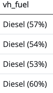


 )
)