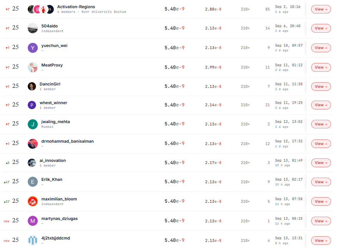
TL;DR. We are a one-person team sitting around rank 10 (public LB 5.40e-9 adjusted, raw final-layer MSE 2.13e-8, C/B 0.2526). We are not going to catch the top of the board, so instead of holding our method until the phase closes we are publishing all of it now, while it can still be useful: the estimator (MIT, github.com/504aldo/whest-p2-cumulant-k3), the five structural facts that got it from the covariance-propagation baseline to the frontier raw error, a per-layer breakdown of where every FLOP goes, and a catalogue of 25 things that did not work, each with a number and a mechanism. If you are between rank 15 and rank 100 and running a cumulant-propagation chain, the dead-end table is probably worth more to you than the code.
Disclosure up front. Every line of estimator code, every probe script and the running findings log this post is written from were generated by an LLM (Claude, Anthropic) in interactive sessions that I directed. I chose the directions, ran every experiment, read every number and decided what to ship. Nothing here is an unverified LLM claim: each statement below names the measurement behind it, and interpretations that were not independently checked are marked “(LLM explanation, not validated)”. ARC’s guidance asks for exactly this transparency; it also asks for methods that are mechanistic rather than tuned, and I have tried to be honest about which of our constants are fitted (section 2.6).
1. Numbers first
The whole trajectory on the public leaderboard, same grader, same 50+50 MLPs. “raw” is the final-layer MSE against ARC’s high-budget Monte Carlo reference; “adj” is the competition score raw x max(0.1, C/B); C/B is metered flopscope FLOPs over the 2^41 budget.
| version (submission) | what changed | raw | C/B | adj | rank when graded |
|---|---|---|---|---|---|
| ARC covariance propagation (kit example, #328319) | baseline | 3.93e-6 | 0.0235 (billed 0.1) | 3.93e-7 | 25/40 |
| V16b (#329389) | factorized K=3 chain in flopscope ops, exact 7 → 4 units per source-layer | 4.46e-8 | 0.4986 | 2.22e-8 | 22/92 |
| V17 (#329480) | + memoryless kappa4 regeneration (one scalar per layer) | 2.26e-8 | 0.4921 | 1.11e-8 | 11/93 |
| V18 (#329531) | + D21 feedback into the birth factors, rank 16 | 2.08e-8 | 0.5093 | 1.06e-8 | 9/94 |
| V19 (#329571) | + exact final-layer trim | 2.083e-8 | 0.4777 | 9.95e-9 | 9/95 |
| V22 (#329584) | + age-gated shared subspace for old sources (rank 384 after 4 transports) | 2.12e-8 | 0.3834 | 8.10e-9 | 7/95 |
| V24 (#329633) | + nested second tier (rank 224 after 7 transports) | 2.15e-8 | 0.3667 | 7.90e-9 | 8/98 |
| V25 (#329644) | + adaptive per-MLP lambda | 2.13e-8 | 0.3667 | 7.80e-9 | 8/98 |
| V26 (#329975) | + Strassen-Winograd block products, 1 level | 2.133e-8 | 0.3455 | 7.37e-9 | 11/112 |
| V28 (#329991) | + residual-time engineering, Strassen 5 levels | 2.13e-8 | 0.2676 | 5.70e-9 | 10/114 |
| V29 (#330093) | + last dense products folded into the batched families | 2.13e-8 | 0.2526 | 5.40e-9 | 8/119 (10/139 on Sep 10) |
Two things to read off this table. Accuracy was won in three steps (V16b, V17, V18) and then never moved: raw 2.13e-8 is where “third cumulant plus a memoryless fourth” lands at 1024 x 16, and our float64 reference chain of the same closure bottoms out at ~2.07e-8 on our 8 local ground-truth MLPs, so the shipped code is within 10% of its own ceiling. Everything after V18 is cost at fixed accuracy: 0.509 → 0.253 x B. The top of the board (raw 1.7-2.0e-8 at 0.145-0.16 x B) is better on both axes, and section 6 says what we know about why.
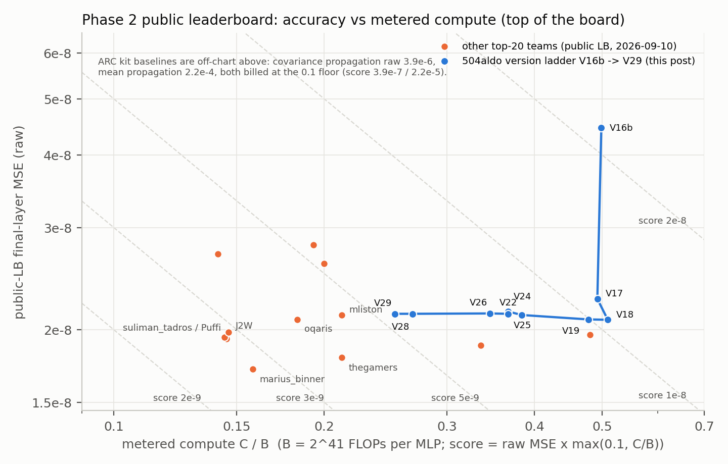
Figure 1. Public leaderboard, accuracy vs metered compute. Blue: our version ladder; orange: the top of the board on 2026-09-10; dashed: score isolines. ARC’s kit baselines are 100x above the top of the plot.
Local numbers, for anyone reproducing: on 8 public MLPs with our own 1e9-sample references (harness/dump_mini_mlps_p2.py), V29 is raw 2.275e-8 at C/B 0.2526 steady; on the 100-MLP mini split through whest run, V25 was 8.17e-9 adjusted (raw 2.23e-8). Our 8 dumps run ~6.5% above the public LB raw at every version, consistently, so compare ratios not absolutes.
2. The estimator in one page
Backbone (known). We use the factorized K=3 cumulant propagation of the companion paper (Wu, Lecomte, Winer, Robinson, Hilton, Christiano, arXiv:2605.05179, S.4.3), with the “K3-simple” term selection of ARC’s reference implementation. In plain terms: instead of sampling inputs, the estimator pushes the STATISTICS of the pre-activations through the network layer by layer. Mean propagation carries the mean; covariance propagation carries the mean and the covariance; K=3 also carries the third cumulant, the object that says how far each layer’s pre-activations are from Gaussian. The ReLU is handled analytically at each layer with the paper’s Wick/Hermite formulas.
The third cumulant is an n x n x n tensor, too big to store, so it is kept as a SUM OF SOURCES. Every ReLU layer injects some non-Gaussianity; that injection is a “source”, born at that layer and then transported through every later layer by the weights. A source is stored in factored form: an n x n propagator leg P (the identity at birth, then P ← W d(w1) P at each layer), an n x n birth leg A = P a_b that carries the covariance at birth, and a few thin n x 16 legs. With 16 layers there are up to 15 live sources, one per birth layer, and this is where the cost is: the paper’s own algorithm needs 30 n^3 L^2 FLOPs = 3.7 x the budget at this shape (its Table 1), which under the hard budget cap means a zero prediction. So the first job was making the same content fit.
The nonlinearity only reads two slices. Of the whole third-cumulant tensor, the ReLU update at the next layer uses just two pieces: the diagonal D3_i = kappa3_iii (one number per neuron, the skewness) and the (2,1) slice D21_ic = kappa3_iic (an n x n matrix). If you feed the chain the exact D3 and D21 it reproduces the exact result (oracle test, F65), so these two objects are the entire interface between “the third cumulant” and “the next layer”. Every design decision below is about producing D21 cheaply and accurately enough. Our fitted rule of thumb: extra final MSE ~ 4.2e-6 x eps^2, where eps is the relative rms error of D21 (two-point fit, F71). Staying within 10% of our 2.1e-8 therefore needs eps <= 2.2%, i.e. D21 must be right to about 2%.
Cost unit. One n x n x n matmul = 2 n^3 = 2^31 FLOPs = 1 unit; B = 1024 units.
2.1 Exact 7 → 4 units per source-layer (V16b, F63)
The reference forms the M leg of each source and transports it. Written out, M = P d(s) + 3 A d(e) + Z L^T where Z is a rank-16 residual leg (randomized range finder at birth, transported like a thin leg). With that, the four (2,1) contributions of a source, D21 = 2H + T2 + T3/3 + 2T4/3 with H = (APw2) A^T, T2 = (AAw2) P^T, T3 = (PP) M^T, T4 = (MP) P^T, collapse into TWO dense contractions per source with right factors A and P: D21 = sum_b LA_b A_b^T + LP_b P_b^T, plus O(n^2 r) thin terms. Per source-layer: 2 transports + 2 contractions = 4 units instead of ~7. Parity with the reference to float32 rounding; C 0.833 → 0.50 x B at identical MSE. This is the single largest cost step and it is exact.
2.2 The fourth cumulant regenerates from the covariance (V17, F68) – the accuracy step
The augmented-K3 chain of the paper carries a per-source kappa4 channel that we could never afford (7 units per source-layer at the ranks that hold accuracy, >= 0.95 x B). Projecting its matrix core G onto live quantities layer by layer, we found
G_off = lambda_l * C_off
with ONE scalar per layer (R^2 0.66-0.97 rising with depth); adding 8 other candidate modes (C*C, Sym(d(mu) K21^T), var var^T, K22, …) changes the final MSE by nothing (2.230 → 2.205e-8). The diagonal of G must stay exact (regenerating it too: 15x worse), and the gain flows through the K4 → K3 feed (the use-side terms alone are harmful, 9.2e-8). With this law the whole (2,1,1) channel is free: raw 4.2e-8 → 2.2e-8 on the lean chain, and V17 halved the LB score at unchanged cost. Why the core aligns with C_off is an open question (LLM explanation offered in the code comments, not validated).
2.3 D21 feedback into the births is rank 16 (V18, F69) and the last layer is cheap (V19, F71)
Of the reference’s V1.6 sub-blocks, only the D21 feedback into the birth factors matters on this chain (-10% raw); it is rank <= 16 (8/16/32 → 2.17/2.14/2.14e-8) and rides on thin transported legs at zero n^3 cost. The final layer emits only the mean, so it needs only var = diag(C_pre), D3 and the kappa4 diagonal: skipping D21 and the full covariance sandwich there is exact and worth 8% of C. But the final-layer skew is essential: D3 := 0 at the last layer is 10x worse.
2.4 Old sources live in a shrinking shared subspace (V22/V24, F72/F73) – the cost step
Transported P legs concentrate with age (rank 128 holds >= 0.92 of the energy after 5 transports, 0.53 at age 1). Sources older than 4 transports are confined to ONE shared basis Qc (n x 384, one randomized range finder per layer on the weighted leg Gram), A_s = Qc FA_s, P_s = Qc FP_s with static factors; sources older than 7 transports move into a nested rank-224 sub-basis inside it. The contraction identity [sum_s LA_s FA_s^T + LP_s FP_s^T] Qc^T keeps one trailing n^2 r product per layer. Measured law: the rank that holds accuracy is ~3n/8 at age 4, n/4 at age 6, 7n/32 at age 7, and one notch lower is a cliff (r = 256 at age 4: +22% raw; r = 128 at age 7: +15%). Cost 0.478 → 0.383 → 0.367 x B for +3.4% and +1.2% raw. One honest note: rank 192 at age 7 looked best on 2 MLPs and was not on 8; the shipped 224 is the 8-MLP optimum.
2.5 Lambda tracks an online observable (V25, F75)
The per-layer lambda is smooth in depth (peak ~1.1e-2 at layers 4-5, 7e-3 at 15) and, per MLP, proportional to mean(kappa4 diagonal)/mean(variance) with log-log slope ~1 at every layer (per-layer r = 0.84-0.99). The rule removes 60-80% of the per-MLP spread of the fitted lambdas and costs one n^2 matvec. Its score effect is small (-0.6% locally, -1.3% on the LB): the table was never the raw bottleneck. Reported because it is a clean mechanism, not because it moved the rank.
2.6 What is fitted, exactly
Everything a judge would call a constant, with its origin and sensitivity: the 16-entry lambda table (least squares of G_off on C_off on 8 public MLPs; global scale 0.9/1.1 → -0.2%/+2.3%), the per-layer reference ratios of the adaptive rule (8-MLP means; a normalization), the exponent BETA = 1 (fit 1.08; 0.8/1.0/1.2 flat), the residual-leg rank 16 (16/32/64 → 2.35/2.39/2.41e-8; higher rank is WORSE raw and costlier), the feedback rank 16 (32: raw -2.5% at +5.9% C, score-negative), the age gates 4 and 7 and ranks 384 and 224 (the law above). The Wick/Hermite term coefficients are the paper’s, exact. No leaderboard number ever entered a fit.
2.7 Cost engineering (V26-V29, F79-F81) – disclosed
V26-V29 do not change the arithmetic (raw identical to four digits on every MLP). They compute the same n^3 products with the Strassen-Winograd block recursion written as ordinary flopscope ops on preallocated buffers (7 half-size products + block additions per level, up to 5 levels, minimum block 32), batched across all sources of a layer as one “family” so that one op covers a whole stack. flopscope bills the recursion at its analytical count; float32 results are within ~1e-6 relative of the dense product and the MSE is unchanged to 4 digits. What gates the depth of the recursion is not FLOPs but the 400 ms residual (non-flopscope) wall-time cap: the residual clock is dominated by result-buffer allocation churn, not by op count (F53) – writing every result with out= into persistent pooled buffers gives a flat ~0.02 ms per op and cut the base chain from 0.331 to 0.170 s (V27), which is what made 5 levels shippable (V28). We asked the sponsor on 2026-09-05 whether Strassen expressed this way is within the fair-accounting rule; no reply as of this post. The #1 team of Phase 1 disclosed the same technique. If ARC rules otherwise, V25 (#329644, no Strassen, 0.3667 x B) is our fallback and the method is unchanged.
3. Where the FLOPs go
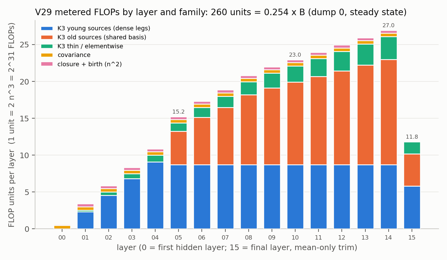
Figure 2. V29 metered FLOPs per layer by family (flopscope namespaces, one public MLP, steady state): 260 units = 0.254 x B.
The ledger (F86): 95% of the bill is third-cumulant source machinery, split 116 units “young” sources (dense legs, at most 4 alive, flat 8.7 units per layer from layer 5 on: 4 sources x 2.17 units under Strassen pricing) and 107 units “old” sources (shared basis, growing ~1.1 units per extra old source per layer), plus 25 units of thin and elementwise work; the covariance costs 7 units and the whole nonlinear closure 6. Engineering headroom inside this ledger is <= 4% on paper and ~0% shippable under the residual cap.
Here is the number that ended our climb. Our bill WITHOUT the old tier is 153 units = 0.150 x B. The leaders’ multipliers on the same day were 0.149 (Puffi), 0.152 (suliman_tadros), 0.164 (J2W). Whatever carries their old-source content costs them ~nothing, while ours costs 107 units for a 6x raw gain (keeping only 4-5 young sources: 1.35-2.9e-7). So the top tier is not a compressed version of our representation, and section 5 says why no compression of ours can get there.
4. The dead-end catalogue
Each row is a measured result at the Phase 2 shape (1024 x 16, 8 public MLPs unless noted), with the mechanism we found. F-numbers are entries in the findings log shipped with the code.
| # | idea | result | mechanism / why |
|---|---|---|---|
| 1 | Drop old sources (window of W youngest) | W=4: raw 1.02e-6; monotone worse as W falls (F61) | every source is needed at the final layer; skipping even one is ~4x (F66) |
| 2 | Memoryless closure: replace old sources by a tensor supported on the (2,1)/(3,) slices | 9.1e-7 = 45x worse (F65) | the next layer’s slices need the fully off-diagonal K3; the lost part is 18-23% of D21 energy per layer, high-rank, not predictable from live-state features (+0.02 R^2) |
| 3 | Puffi’s Phase 1 “A716” slice/response-series closure rebuilt at this shape | 9.8e-7, the same floor (F82) | same mechanism as 2; the 144-constant fitted transported correction buys 1.07x |
| 4 | Gaussian scale-mixture closure on the fluctuation part | 2.33e-6 (F78) | misses the kill line by 2.3x; the non-Gaussianity is not a mixture |
| 5 | Capped hub columns (“atoms”, CP-rank cap on the merged tensor) | cap 4n columns: D21 relative error 0.39; 8n: 0.03-0.14; need 0.02 (F76) | column importance is flat (top quarter = 73% of mass) |
| 6 | Symmetric Tucker confinement of all three legs | R=512: 14x, R=256: 31x (F46) | the P leg is born as the identity: full rank at birth |
| 7 | Per-source rank ladder (lower rank for older sources, separately) | 17x accuracy loss for 1.8x compute saved (F55) | see the age law: below it is a cliff, and separate bases pay a full range finder each |
| 8 | Shared basis below the age law (age 3 at r=256, age 2, r=128 at age 7) | +96%, 3x, cliff (F72/F73) | the propagator spectrum decays with age exactly as fast as the law says, no faster |
| 9 | Per-source kappa4 legs (the paper’s augmented K=3) | dense floor 7 units per source-layer, >= 0.95 x B (F58/F64) | the third dense leg of the kappa4 channel is irreducible; the regeneration law (2.2) gets 90% of its value free |
| 10 | Learned / online output corrections (ridge on live features, per-layer mean correction) | final-layer features correlate < 0.09 with the error; 1.01x on the regen base (F46/F47/F68) | the residual is high-order in the input and uncorrelated with cheap features |
| 11 | Cheap covariance propagation + skew/kurtosis fixes (marginal Edgeworth, Gram-Charlier co-skewness, exact Mehler off-diagonal) | capped at 4-5e-6 (F60) | order 2 plus marginals cannot see the cross-neuron third cumulant |
| 12 | Monte Carlo control-variate hybrids on top of the analytic chain | needs 33-300x variance reduction, best realizable 1.5x (F62) | same as 10: nothing cheap correlates with the residual at depth 16 |
| 13 | Symmetric-contraction FLOP tricks (Schatz / Solomonik-Demmel) | do not apply (F67) | no dense symmetric order-3 object is ever formed: every contraction is a non-symmetric matmul on leg matrices |
| 14 | Accounting levers (symmetric tags, dtype tricks) | none: flopscope billing is tight (F49/F56/F64) | (A*c)@A.T bills full; f16 is billed as f32; einsum is billed at naive contraction cost |
| 15 | float32 → float64 hot path | +0.004% (noise) (F88) | there is no precision loss to buy back; all error is closure/truncation |
| 16 | Higher feedback / residual ranks, two range-finder passes | raw -1..-3% for +3..8% C: all score-negative (F75/F88) | the eps^2 law: D21 is already at ~2% |
| 17 | Exact (2,1,1) kappa4 core instead of the regeneration | -9% raw at 0.5-1.0 x B (F58/F64) | see 9 |
| 18 | Tucker core of the merged old tier in the shared basis | costs r^3/n^2 units for the tier: 10.7 u at r=224, 54 u at r=384 > today’s 6-14 u (F88) | wins only below r~150, under the accuracy cliff |
| 19 | Hub-side merge of old sources into fewer columns | = row 5 (F88) | CP-rank reduction with flat importance |
| 20 | Adjoint / backward sensitivity of the final mean to D21 | no cost drop (F88) | still one dense contraction per (source, layer) pair, and it linearizes the feedback of row 2.3 |
| 21 | Any Hadamard product of factored legs | Khatri-Rao rank r^2 (F71) | forming a leg from the basis costs what transporting it costs; this is THE wall of section 5 |
| 22 | Sampling variants that won Phase 1 (QMC, antithetic, preintegration, Stein CVs) | at 1024 x 16 pure sampling sits at ~1.2e-6 adjusted (the “vs sampling” column) (F42) | analytics beat sampling by 200x here; MC is at most a floor-priced sidecar |
| 23 | Pricing polish (Strassen on the join’s 60 lone products, AGE_OLD 4->3, composite rotations) | <= 4% on paper, 0% shippable: +74-118 ms residual against a 400 ms cap (F86) | ~0.1 unit saved per ms of residual, the base residual is 0.25-0.34 s |
| 24 | Literature: four triage passes, ~25 papers (finite-width corrections, uncertainty propagation, cumulant tensors, Edgeworth, tensor programs) | zero methods (F70, F83-F85, F87) | the finite-width literature is annealed over weights (odd cumulants vanish by construction); the quenched literature stops at covariance |
| 25 | Everything above, repackaged | the V29 chain is at its raw floor; no leg-based representation of this expansion reaches 0.15 x B (F88) | – |
Triage rule we ended up with, in case it saves you a week of reading: (1) is the paper annealed over weights? then kappa3 = 0 by construction and it is a citation at most; (2) if quenched, does it ever write a cross-moment of order >= 3 among distinct neurons? if not it cannot touch the objects above; (3) for cost papers, does the saving act on a factored representation or only on a dense n^d tensor you never materialize? (4) does it report moment error vs depth at <= 1e-6, or nothing?
5. The wall, stated once
Every source enters the next layer through Hadamard products of its own legs, AP, PP, A*A, contracted against a third leg (the (2,1) slice of Sym(X x P x Y) with two indices identified is sum_q X_iq P_iq Y_cq). For factored legs A = Q FA, P = Q FP the Hadamard product has Khatri-Rao rank r^2, so it cannot be done in factor space, and forming the dense leg from Q costs n^2 r, exactly what transporting it costs. The shared basis is therefore a 2x-per-source lever, never a 10x one: old sources are re-formed and re-contracted every layer. The bill is set by the number of dense n x n legs formed per layer (8 young + 2 x 10 old at layer 14), and nothing in the pricing changes that count. We closed the three “open doors” of this argument (a Tucker core in the shared basis, a multiplicatively closed basis, a hub-side merge) by arithmetic in F88.
6. What we think the top of the board is doing (honestly: we do not know)
Two facts. The leaders’ bill equals ours minus the old tier, to three digits. And the new #1 (marius_binner) has raw 1.71e-8 at 0.158 x B, below the ceiling of “K3 + memoryless kappa4” that our float64 chain measures at ~1.94e-8 on the LB scale. So the top methods carry fourth-cumulant content beyond a memoryless core, AND old-source content, at roughly the cost of our young tier alone. Nothing in the paper, in the reference code, in Phase 1 public write-ups (Puffi’s lineage measured dead here, rows 3 and 5), or in the literature we read does that. Our best guess (LLM explanation, not validated): it is not a per-source hub-tensor expansion at all. If anyone at the top writes theirs up after Oct 17, this catalogue says which tricks it is NOT.
7. Practical notes on the Phase 2 grader (the things that cost us submissions)
- The 5 s setup cap fails the ENTIRE submission, not one MLP. Load nothing heavy at import.
- NumPy is not installed at eval time; stdlib + flopscope only. Our estimators are single files with the tables embedded.
- Dataset weights arrive as float64 and float64 is billed at 2x. One astype(float32) per MLP before the hot loop.
- The grader’s smoke test uses NON-suite shapes (we saw depth 32). Gate every shape-specific branch on (n, L) and keep a plain fallback path.
- The FLOP budget is a hard cap: C > B is a zero-prediction fallback for that MLP with no discount, not a score multiplier above 1.
- Residual wall time (400 ms per MLP) is dominated by result-buffer allocation, not by the number of ops. out= into preallocated buffers gives a flat ~0.02 ms per op. Memory: keep the buffer pool bounded; ours peaks at 5.5 GB after two predicts against an 8 GB limit.
- The first predict of a process is slower (pool warm-up). We run the first MLP at a shallower Strassen level; the grader’s per-MLP compute is the steady-state number.
- flopscope bills einsum at the naive contraction cost with no symmetric discount; matmul forms of the same contraction are often cheaper AND faster in residual time.
- The public score is exactly raw x C/B of the steady state; local
whest run --split minireproduces it to ~5%. - One physical core at eval: test with restricted threads; local 24-thread timings are meaningless for the caps.
8. Reproduce it
Code: github.com/504aldo/whest-p2-cumulant-k3 (MIT). estimators/estimator_v29.py is the live best and estimator_v25.py the same method without Strassen; each version is a self-contained file, and generators/make_vNN.py are the asserted textual patches from one version to the next, i.e. the change log is executable. harness/ has the 8-dump ground-truth builder and the measurement scripts; lean/ is the float64 torch reference chain every closure experiment ran on (it imports ARC’s reference term tables). docs/ contains the ablation table (every version on the same 8 MLPs, mini and LB), a claims-with-evidence list with a hedge label per claim, and a derivation-to-code map from the paper’s equations to the code blocks. Toolchain: flopscope >= 0.12, whestbench >= 0.16, dataset revision v2-phase2.
If you use any of this, a reply here saying what worked or did not would be the best outcome of the post. Good luck to everyone still climbing.
504aldo (solo, Independent). Findings F-numbers refer to docs/findings_log.md in the repo (the raw, append-only research log, ~90 entries; docs/findings_index.md is its table of contents).