"Asymmetric" loss function?

Hey everyone,

I’ve been low-key obsessed by the fact that my loss function was somehow “asymmetrical”.

Basically, I don’t really mind overcharging a risk from time to time. Worst case scenario is I don’t sell the quote.

What I really don’t want to happen is undercharge a car or a city because no one from my portfolio who owned that car made a claim. Then I charge them too low, I get adverse selected to death.

Is there a way to take this into account? Maybe a custom loss function like RMSE, but you double the cost when you predicted under the actual amount? Not sure how I’d implement that though.

I just had an idea while walking earlier tonight. It might be absolutely stupid, but I posted it here anyway.

2 Likes

RMSLE is one of the asymmetric loss functions but I have not explored further in it.
Two characteristics:

  • RMSLE is greater when the model underestimates

  • Due to the log, it is more robust to outlier (which can be a bad / good thing?).

5 Likes

First of all less risk less expected reward.
You could try some old-fashioned credibility - no car details in portfolio or not in urban area means greater loading. This is easier on commercial lines eg Employer’s Liability but should be applicable to motor insurance.
Also thinking about this algebraically, you are actually asking:1) how can you quantify how lonely or distant future policies are from your current portfolio 2) whether extrapolation is required and is interpolation possible and reliable.
This sounds like distance measures in Algebra and some sort of density measure.

that’s new to me - thanks!

That’s a great topic !!

During the competition I did something similar to you, for instance on the vehicle IDs, I decided to “cap” all the effects below -5% (and refitted the model) as illustrated for some vehicles in the graph below:


The dashed green line represents the “optimal” coefficients in term of predictiveness while the full line represents the coefficient in the model used in the pricing ; for the two levels with the arrows, the “statistical” model was having effects stronger than -5% (dashed line) but I capped the effects at -5% (full line).

This is just a very dirty actuarial cooking but the idea is the same as you : “in case of doubt, I am happy to increase the price but not happy to decrease it”.
A cleaner approach (where you assess the variance of your predictions for each profile and charge a buffer depending on it) would clearly be much better but I don’t know any research on this ; I don’t have a clear motivation for this approach, providing a formula for this buffer. Does someone know any paper with a real, rigorous and formal version on this topic ?

2 Likes

I tried looking into this for the competition, but I didn’t delve too much into the theory. Quantile regression was one approch i found being discussed (and a quick search shows lots of theoretical papers describing it in more detail). Another approach is to use bagging to estimate the variance (basically fitting lots of models on samples from the data). This is the approach i followed. There is also some theoretical literature on this, but i didn’t look into it too much detail at the time. Doing some searches, this article gives some theoretical discussion on the approach: https://arxiv.org/pdf/1908.02718

1 Like

Interesting!
What did you do with your premium once you had your final prediction and a couple more predictions to assess variance?

Here’s how I imagine this.
I have a model trained on 100% of the population and 5 others models trained on 40% samples of the population with replacement. (I could also just reuse the 5 models I already trained for cross validation)

Person A is predicted a 200$ claim by the “main” model and 180,190, 200, 210 and 220$ by the small models.

Person B is also predicted a 200$ claim by the “main” model, byt 140, 170, 200, 230 and 260$ by the small models.

Clearly, I want to charge person B more. My understanding from your comments is that there is no set formula in the actuarial world for that. Guess we’ll have to simulate it… :slight_smile:

1 Like

Thanks for sharing!

I also had an “other” category in my model for cars that were less frequent, but there’s a lot of different cars in that category, many of which probably have wildly different expected claims.

I’m also very interested on something to account for the uncertainty around a single premium.

­Coming up with a premium from an estimate of the mean and variance of each risk is not easy. I’m guessing it might be possible to some up with some game theory approach for solving the problem to minimize the winners curse, but I just took a more empirical approach of checking the premium I charged exceeded the claims with a high enough probability.

I originally started loading all estimates of the mean with 2 times the standard deviation, but I was getting a lot of large claims in the weekly competition. I did some analysis and found the coefficient of variation was generally quite high when the mean expected loss per policy was low, and it was low when the mean was high. I found this a bit counter-intuitive at first, but it makes sense because a low mean is associated with a low frequency, so there is a greater chance of claims being 0, which is far from the mean. I had to adjust the loadings from a flat number of standard deviations to prevent undercharging high frequency policies and overcharging low frequency policies.

The influence of claim frequency on the variability estimate is probably the main disadvantage of using a variance approach – the variance is heavily influenced by results being better than expected, so it doesn’t really give you the asymmetric measure you were originally looking for.

1 Like

That’s super cool!

Doesnt really have to be an “asymmetric loss function”, just something that reflects the fact that I’m more careful when giving rebates than when I am charging more.

Your model ended up loading a higher percentage to policies with lower predicted claims and that works with the spirit of what I’m looking for :slight_smile:

As a percentage of the premium, what did 2 times the standard deviation typically represent on an average premium of 100$ ?

When expected claims were 100 the average standard deviation was about 6, so 2 standard deviations was about 12. The graph below shows how the average standard deviation varied as the expected claims increase.
image

There were a small number of policies where the standard deviation was quite high compared to other policies with similar levels of expected claims. This is a density plot of expected claims cost versus standard deviation, with green being the lowest density of policies and blue being the highest density.
image

And a zoomed in version of the plot:
image

2 Likes

really nice work!
12% seems pretty low compared to what most folks ended up charging. I’ll go back to the solution sharing thread to see if you posted your final % :slight_smile:

12% is low. I started with a loading of 2 standard deviations, but I ended up modified the loading, eventually ending up with an average loading of just over 30%, with lower loadings on policies with low standard deviations.

1 Like

Thanks @Calico that’s really nice :slight_smile:

I wanted to dig into this topic a bit for years; this forum gave me the opportunity to do so :slight_smile:
So I tried to model what the optimal strategy would be and how it changes based on the uncertainty in the model.

I used a very simplistic framework to try to keep things clear.
I supposed :

  • there is an (unknown) risk attached to a policy, called r (say, r=100). The insurer has an estimate of this risk, following a gaussian around it : \hat r=Normal(r, \sigma) .
  • there is a known demand function depending on the offered premium \pi : d(\pi) = logit(a+b \times ln(\pi))

In this situation, the first conclusions can be derived :

  • for every price \pi a real profit B(\pi) can be computed (but it is unknown to the insurer as the real risk r is unknown : B(\pi)=d(\pi) \times (\pi - r) ).
  • an approximation of this real profit can be computed : \hat B(\pi)=d(\pi) \times (\pi - \hat r) ; interestingly it is an unbiased estimate (but using it for price-optimization purpose very quickly lead to funny bias ; I won’t focus on this here)
  • it is quickly clear that most of the computations we can do will not lead to a closed formula ; the reason for that is because the real optimum (solving \dfrac{dB(\pi)} {d\pi}=0 ) does not lead to an explicit solution, I think. So all the results here will be based on simulations.

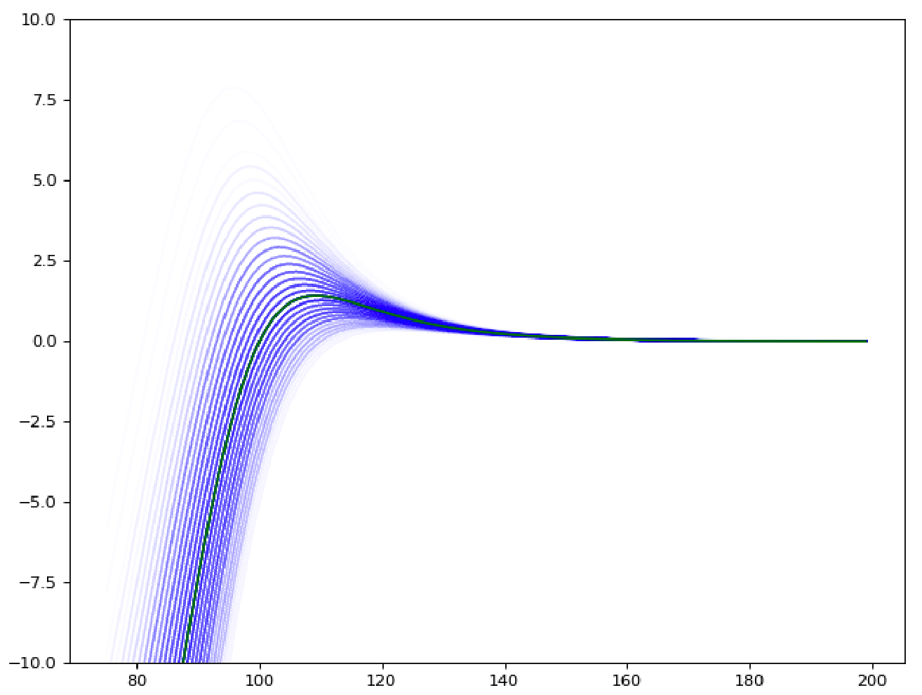
For instance in the graph below (x axis : premium \pi ; y axis : expected real profit B(\pi) - in green - or estimated profit \hat B(\pi) in blue, for different values of \hat r) provides an view of the truth and the estimated truth according to the model.

The question raised by @simon_coulombe is : given an estimated risk \hat r and a known variance in this estimate \sigma, what is the best flat-margin (called m) to apply, in order to maximize the expected value of the real profit : m^*=argmax_m E(B(\hat r \times (1+m))) ?

The intuition we all shared is that it should increase with \sigma. @Calico suggested it should be linear.

As there is no obvious formula answering this question, I ran simulations, taking an example of demand function (a=64, b=-14), a real r (100), and varying \sigma, running 1000 simulations with different \hat r every time.

For every value of sigma, all values of the margin m were tested and the one driving the highest profits B(\hat r \times (1+m)) on average over the 1000 simulations of \hat r was found.
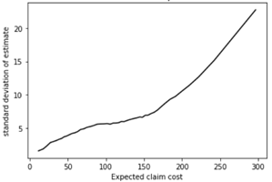
The optimal margin m increases as expected when \sigma increases, as one would expect :
image
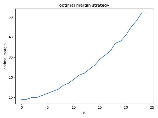
(the values are rounded and there is some noise around \sigma = 20 but it looks more or less linear, indeed).

The profit goes this way :
image
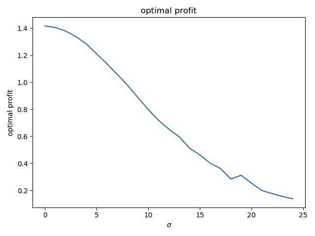
(if the real risk r is exactly known - \sigma = 0 -, a profit of 1.42 can be obtained. If \sigma goes to infinitly large values, the profits tends toward zero.)

This simple test raises a lot of questions that I would like to investigate more seriously in the future :

  • is the optimal margin really linearly increasing with \sigma ?
  • if I use a noise that is not gaussian, what will be the relation ? Maybe there is a distribution of the errors that helps the maths ?
  • in this toy example, the demand function was supposed to be known ; what happens if it also contains errors ?
  • how can I estimate the model errors (it is very hard for the risk models, but probably much harder for the demand and price-sensitivity models !!)
  • strategies optimizing naively the estimated profits \hat B(\pi) built from the estimated risk \hat r are known to be a bad, leading to over-estimated profits and suboptimal pricings ; can a simple correction factor be applied, and how does it relate to \sigma ?

So to summarized, this test kind of confirms the intuition is more or less true, but opens many more questions !! If anyones has some papers on this topic, I would be really happy to get more serious insights !

2 Likes

Interesting analysis. The paper I posted in ye olde library is somewhat connected. It considers the case of a number of insurers with different estimates of a risk and applying the same profit loading, and concluding that if they want to achieve their desired profit margin they need to add a multiple of the standard deviation of the error in their estimates. Its not quite the problem you are aiming to solve, but it might provide some insight.

The problem you outline seems a very difficult one to solve. You might need to write a paper to start the literature :slight_smile: . One potential problem is that it would be difficult to model the demand curve if competitors are using different types of feature engineering, or using additional data that is not available to you. I don’t know how it would be possible to model the potential anti-selection effects from these types of unknowns.

1 Like

wow… wow!

Thanks for taking the time to dig into this and share your results. I’ve only been cheerleading so far, but all the work you and @Calico have shared is really interesting :slight_smile: Super cool to have Calico’s initial idea of linear increase show up in @guillaume_bs 's simulation.

I’m trying to come up with a simulation where there are 2 insurers and 2 groups of clients. Group A and B have the same average, but group B is much more variable. One insurer is aware of that, but the other is not. How bad is the unaware insurer going to get hurt? I’ll let this marinate for a bit :slight_smile:

1 Like