🚃🚃 Train Close Following

:memo: 
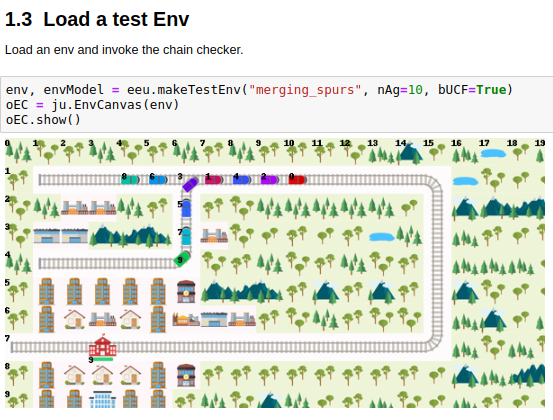
TL:DR: We have improved the way agent actions are resolved in Flatland, by fixing corner cases where trains had to leave an empty cell between each others. This new way to handle actions is the new standard, and will be used for Round 2.

Many of you are aware that Flatland agents cannot follow each other close behind, unless they are in agent index order, ie Agent 1 can follow Agent 0, but Agent 0 cannot follow Agent 1, unless it leaves a gap of one cell.

We have now provided an update which removes this restriction. It’s currently in the master branch of the Flatland repository. It means that agents (moving at the same speed) can now always follow each other without leaving a gap.

Why is this a big deal? Or even a deal?
Many of the OR solutions took advantage of it to send agents in the “correct” index order so that they could make better use of the available space, but we believe it’s harder for RL solutions to do the same.

Think of a chain of agents, in random order, moving in the same direction. For any adjacent pair of agents, there’s a 0.5 chance that it is in index order, ie index(A) < index(B) where A is in front of B. So roughly half the adjacent pairs will need to leave a gap and half won’t, and the chain of agents will typically be one-third empty space. By removing the restriction, we can keep the agents close together and so move up to 50% more agents through a junction or segment of rail in the same number of steps.

What difference does it make in practice?
We have run a few tests and it does seem to slightly increase the training performance of existing RL models.

Does the order not matter at all now?
Well, yes, a bit. We are still using index order to resolve conflicts between two agents trying to move into the same spot, for example, head-on collisions, or agents “merging” at junctions.

This sounds boring. Is there anything interesting about it at all?
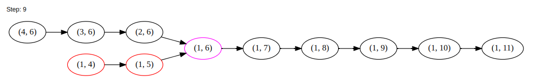
Thanks for reading this far… It was quite interesting to implement. Think of a chain of moving agents in reverse index order. The env.step() iterates them from the back of the chain (lowest index) to the front, so when it gets to the front agent, it’s already processed all the others. Now suppose the front agent has decided to stop, or is blocked. The env needs to propagate that back through the chain of agents, and none of them can in fact move. You can see how this might get a bit more complicated with “trees” of merging agents etc. And how do we identify a chain at all?

We did it by storing an agent’s position as a graph node, and a movement as a directed edge, using the NetworkX graph library. We create an empty graph for each step, and add the agents into the graph in order, using their (row, column) location for the node. Stationary agents get a self-loop. Agents in an adjacent chain naturally get “connected up”. We then use some NetworkX algorithms:

  • weakly_connected_components to find the chains.
  • selfloop_edges to find the stopped agents
  • dfs_postorder_nodes to traverse a chain
  • simple_cycles to find agents colliding head-on

We can also display a NetworkX graph very simply, but neatly, using GraphViz (see below).

Does it run faster / slower?
It seems to make almost no difference to the speed.

How do you handle agents entering the env / spawning?
For an agent in state READY_TO_DEPART we use a dummy cell of (-1, agent_id) . This means that if several agents try to start in the same step, the agent with the lowest index will get to start first.

Thanks to @hagrid67 for implementing this improved movement handling!

3 Likes

Thank you @ hagrid67 very good job. I think the graph (network) can also be used to create new RL observations. How can i run a demostration of the graphic structure, do you have an examples with illustrative rendering?

Hey Adrian - there is an example in the notebook Agent-Close-Following.ipynb.
It sets up a little test env, runs a few steps / actions, and renders the chains / trains of adjacent agents using GraphViz.

image

At step 9 you can see that the agents in cells (1,4) and (1,5) are blocked by the others in front, and the lower-index agent in (2,6). (I couldn’t find an easy way to make GraphViz render the agent numbers in the cells, as well as the row, col node identifiers :slight_smile: )

For the “close-following” (aka unordered close following or UCF) we set up a digraph for every step, and the edges are the moves the agents want to make. This is of course different to creating a (static) graph or digraph for the rails.

Apologies to anyone struggling to install GraphViz btw. If it proves to be a problem we will improve our instructions. GraphViz is not necessary for the operation of the env but it was useful for making the graphical test cases.

Hey, is current Round 1 using master branch’s version, or pip release 2.2.1?

Very nice - thanks @hagrid67 . This graphic looks excellent. It could help to improve RL. Because we can see “flows” of agents in a very precise way. And we may be able to include this information into tree observation. The current tree observation just scans forward (in the direction of travel), but now we can also get information about the incoming traffic at switchs in very accurate way. This might be important information to avoid overfilling which can lead into “unpredictable” deadlocks (traffic jam issue).

@hagrid67: Do you also have a illustrative (screenshot) image with agents travelling in different direction? And with more then one junction (join and split)?

Hi, it is using older version for Round 1 i.e. no change in evaluation.
New version will be released ~together with Round 2.

1 Like

Hey @adrian_egli, sorry just seen this.

I made a simpler way (I think) to create test cases using some logic from the editor, allowing you to paint “strokes” (like mouse or brush strokes) on the env. It isn’t perfect but I think it’s easier than assembling rail junctions by number and rotation; also in a way it’s easier than the editor because (1) no extra files involved and (2) it was always a bit tricky to add agents using the editor.

It’s in env_edit_utils.py (this example is not yet committed):

   # two loops
    "loop_with_loops": {
        "llrcPaths": [
            # big outer loop Row 1, 8; Col 1, 15
            [(1,1), (1,15), (8, 15), (8,1), (1,1), (1,3)],
            # alternative 1
            [(1,3), (1,5), (3,5), (3,10), (1, 10), (1, 12)],
            # alternative 2
            [(8,3), (8,5), (6,5), (6,10), (8, 10), (8, 12)],
            
            ],
        
        # list of row,col of agent start cells
        "lrcStarts": [(1,3), (1, 13)],
        # list of row,col of targets
        "lrcTargs": [(2,1), (7,15)],
        # list of initial directions
        "liDirs":  [1, 3], 
        }

(you need to remember to overlap the strokes a bit, otherwise they will not join properly)

test

1 Like

@hagrid67 I like your render image. Do you mind to tell how you make the agent ID showing on the plot?

Hi, there’s an option show_debug when you create the RenderTool. Set it to true. And the row/col numbering is show_rowcols - but here the option appears in RenderTool.render_env.

Sorry for the inconsistency…