That’s exactly what I did. And I thought I had said too much here, about busting the server memory trying to handle all the models 
Lots of really clever ideas there - good job!
We discussed this offline, might as well add my comments here 
This is the part I’m really wondering about. My understanding is that you calculated a frequency for each city, then “pulled” toward the global average. Cities with less exposure would be pulled more than cities with big exposure. What’s the formula for that?
I was thinking about using a “poor man’s bayesian” approach. Basically I would calculate a frequency for all the cities, but for each city I would add (say) 50 years of exposure and the number of claims I would get at the global market frequency. If the global frequency is 0.10, then I would add 50 years of exposure and 509 * 0.1 = 5 claims to every city. A small city with 4 years of exposure and 1 claim would have a “bayesian” frequency of 1+5 claims over4+ 50 years, so 0.11 , while a larger city with 400 years of exposure and 100 claims would have a “bayesian” frequency of 100+5 claims over 400+50 years, so 0.233, aymptotically trending towards 0.25.
Oh! I just had another idea. I’ve been looking for a way to incorporate that my loss function is asymetric: I don’t mind overcharging ( I just lose a sale), but I really don’t want to undercharge and be the victim of adverse selection because the only person from that city in my portfolio never made a claim. In other words, I really want to charge you more if you are in a “risky neighbourhood with small exposure” but I dont necessarily want to give you a rebate if you are in a “safe neighbourhood with a small exposure”.
One way to do this might be to have a larger offset when I your frequency is lower than the market average. Like if you are over the average frequency my offset is 5 claims and 50 years (like above), but if you are under the average my offset will be 10 claims and 100 years, so it’s easier to bring my price down.
Here is the modeling approach I took. I had tested several models but ended up with QDA and Linear Regeression.
-
Use binary logistic regression model to predict the likelihood of a claim and a linear regression to predict the severity.
-
Resample data for logistic regression: I oversampled policies with claims and under-sampled policies without claims.
-
Resample data for linear regression: We could use the same resampled data from #2 above, but I prefer to resample again since it has been proven to have a better performance with different samples/subsets of the same data. There are 2 ways to resample for linear regression:
a) Only use data where “claim amount” > 0. This is the most common approach but it overstates the amounts as every new policy will have a “claim amount”.
b) Use policies with “claim amount” > 0 but add some polices with “claim amount” = 0. This is my preferred approach but there will be instances when the “predicted claim amount” will be less than 0. It is not possible to have claim amount less than 0 so will need to be adjusted.
-
Determine the threshold to be used for the predicted probabilities and predicted severity from the 2 models. I look at the distribution of the test data to determine the threshold.
-
Predict claim amount: This takes the data from #4. What we are looking for is to have the income that is close to losses (income = plus/minus 10% of the losses).
-
Predict premium: This is usually a trial and error for the first few weeks but we should be able to come up with a good figure based on our market share and profit/losses. I started with 3* claims + (some constant) and had 25% market share but more large claims. In the following week, I increased the premium to 4* claims which reduced the market share and large claims that resulted in higher net profits.
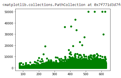
My goal was to write the polices in middle. Not the cheap ones with no claims or the expensive ones with lots of larger claims. This is my model on training data. X is price and Y is claim amount.

if the overall average was .11 and the city had .2 but only 200 observations but I require 400 observations to fully trust it, I’d set Z as sqrt(200/400) and make the weighted average as Z * .2 + (1 - Z) * .11, then cluster based on the weighted average. I wasn’t very scientific with selecting the requirements to fully trust the number but I did try varying it and checking what values resulted in clusters that improved CV fit.
that makes sense - thanks!
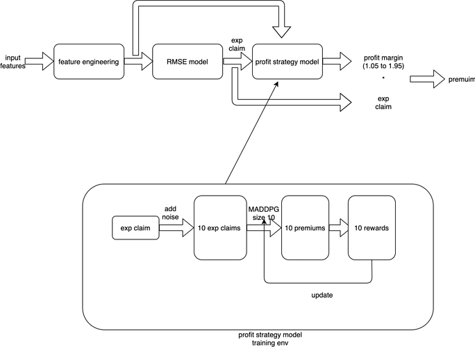
HI we used deep reinforcement learning(MADDPG @openAI 2018) to simulate the market environment and try to get a best strategy in a very unstable market. This is our brief summary. Here we focus on the profit strategy part since we find claim prediction is a high-variance problem(we add gaussian noise~N(0,15) and the RMSE almost does not changed, see 1.3).
1. analysing part
1.1 market summary analysing
| leaderboard average profit per invoice | our average profit per invoice | expected factor(1+profit margin) of market | expected money of RMSE model in market | |
|---|---|---|---|---|
| week9 | N(-4,10) | -1.5 | N(1.25,0.25) | N(115,25) |
| week10(predicted) | N(-1.5,9) | N(1.5,0.25) | N(115,25) |
leaderboard average profit per invoice is calculated from the leaderboard(see appendix), and expected factor(1+profit margin) of market and expected money of RMSE model in market is calculated from the market simulation experiment(this is a analysing in week9 and in week10 the average market profit is far more different than that we predicted in week9 haha)
the factor(1+profit margin) of all 10 agents in RL model after training obeys distribution~N(1.8,0.26), so i think the 80% profit margin will probably be a Nash equilibrium in this market simulation.
1.2 the relationship between our profit margin and average profit margin of market
something wrong here, I cannot upload table…but we find the best profit margin=market average profit margin-0.3(if market average profit margin is larger than 0.3)
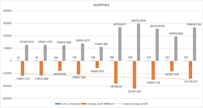
here to test the RL model performance we put the best one(choosed from 10, and we call it king model) in the simulated market and try to use any methods(like changing the profit margin of other competitors) to attack this king model and finally we find this king model can make sure to profit(at least dont loose money) in any environment with a average profit of 1.15 per invoice in hundreds of experiments. But we know the real market/compitetion is much more complex and competitive than our simulated market and most likely our profit depends on the profit strategies of other 9 companies(you cannot expect too much in a very bad market) so we dont expect too much.
1.3 why it is a high variance problem
here we add a gaussian noise with different std to test how random noise affects the result.
| noise std | validation RMSE |
|---|---|
| 0 | 827.74 |
| 15 | 827.76 |
| 20 | 828.1 |
| 25 | 828.15 |
so we think the claim prediction problem is a high variance problem as shown in the form.
2. inference pipeline
reference:
here i think the better way is using 10 different models to simulate the market environment as @michael_bordeleau but that would be much more complex so we did not do that.


