It was very edifying to finish 3rd in this competition alongside some very strong competition.
My approach was to be as data-driven as possible and make extensive use of GBMs. I had a good validation strategy and I was very conservative about allowing small improvements to avoid hill-climbing my internal CV score. I biased my decision-making in favour of dropping features and applying monotonicity constraints where appropriate.
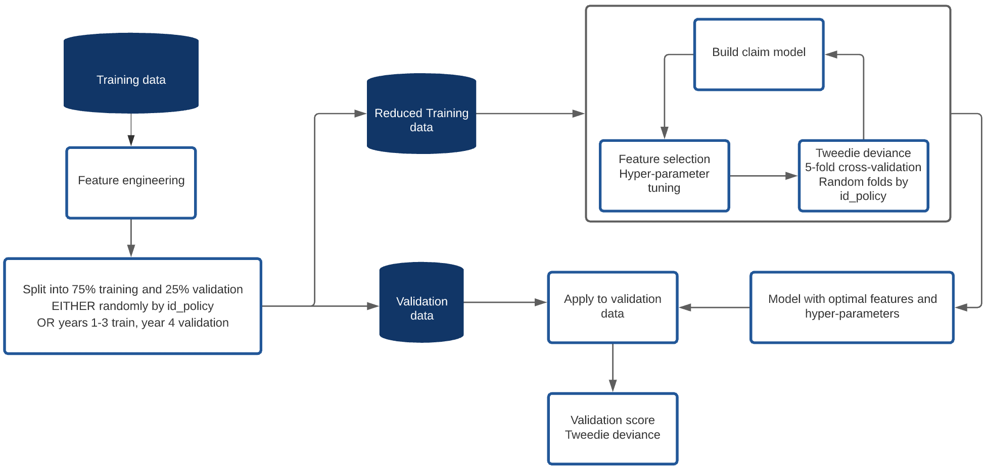
This was my model pipeline:
I coded up a lot of features but was strict about which ones actually were added to the models I built. Other than the raw features we were given, I included the following:
- Flag for locations with population < 20 or count < 4 (location defined as unique combination of population and town_surface_area)
- Count of location in training data
- Oldest and youngest driver ages, license lengths, sexes
- Vehicle momentum (speed * weight)
- Vehicle value adjusted for age of vehicle
- Count of vehicle
- Location target-value encoded features
- Vehicle target-value encoded features
- Vehicle year of manufacture (year - vh_age)
- NCD against par for age
- Age difference of drivers
- Features based on claims history and evolution of NCD for policies in the training data
I tested a lot more!
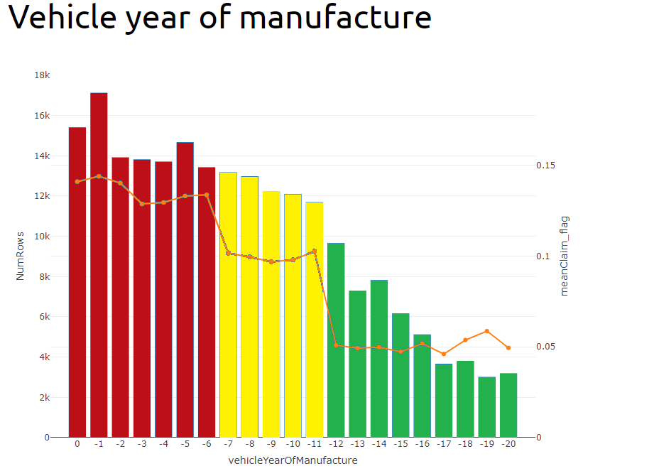
I said in my presentation that vehicle year of manufacture was my strongest variable. In fact, because I one-hot encoded pol_coverage into four variables, one for each level, when you re-combined their importances, pol_coverage was still the most predictive factor, but vehicle year of manufacture was not far behind and I got used to seeing it at the top of the list (and before I coded it, vh_age was top).
I was very surprised by how strong a predictor vehicle year of manufacture was. I don’t understand why vehicles manufactured in year -11 are twice as risky as vehicles manufactured one year before in year -12. I feel this must be some artefact of the way the data was put together - maybe it was extracted from three different sources and combined? I would be very interested to hear from the organisers as to why this factor should be as predictive as it was!
For dealing with year 5 pricing on policies where we had claims history, I augmented the training data by including each row twice, once with all the claims history set to missing, and once with the claims history features populated. (Technically I only included rows from year 1 once since either way there was no history). The features I used were, number of years with claims over the last n years, total amount claimed in the last n years, change in NCD over the last n years, etc.
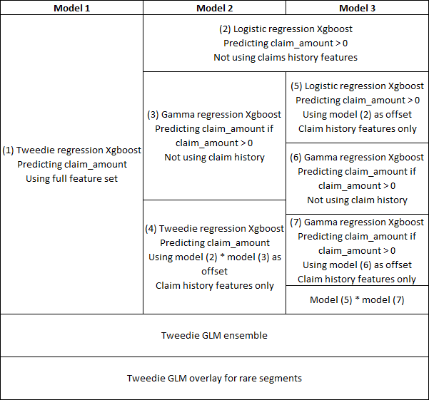
I tried lots of different model structures and feature sets in the hope of getting a sharper final model by ensembing a range of diverse models. In the end, as I only used XGBoost, they tended not to be that diverse, or the ones that were diverse did not add much to the ensemble, of which only three made it.
My final structure is below:
I did not make many underwriting judgements or overlays but I did put in a discount for hybrid vehicles as the model was over-estimating the claims costs for them, I also had a discount where both drivers were female and loads where both were male as well as loads for quarterly payment frequency and pol_usage being “AllTrips”.
In the end I think I was probably very strong pricing policies that were in large homogeneous segments where there was plenty of data for xgboost to work its magic and potentially poor in areas where there were less data and more UW judgement might have been appropriate. I also don’t think I paid enough attention to the pricing element.
I tried to load my prices so that I was comfortably in profit, but also writing policies across the full range of premium values, from small to large.
On the whole it was a very rewarding experience and I enjoyed hearing how differently other people approached the same problem. In the end there were only a few teams that managed to write a significant market share while remaining profitable and I was very pleased to be among them.